Bob Hall and Consumption

I wrote this essay on Bob Hall and Consumption (link goes to pdf on my webpage) for the conference in honor of Bob Hall at Hoover, November 22. It turned into a more extended history of some trends in macroeconomics, which any student of macroeconomics might find useful. Why we do what we do is often obscure. If this post exceeds your email limit, finish on the website at grumpy-economist.com

---

Bob Hall and Consumption¹

I’m going to cover just two of Bob Hall’s many pathbreaking papers, “Stochastic Implications of the Life Cycle–Permanent Income Hypothesis,” Hall (1978), and “Intertemporal Substitution in Consumption,” Hall (1988), both in the Journal of Political Economy. Along the way, this turns in to a brief history of the emergence of modern macroeconomics, and one of its central unsolved problems, intertemporal substitution.

I titled my remarks at the conference, “Consuming Hall at Chicago.” I think you know Hall has many fans at Stanford, but you might not know just how popular Bob was at Chicago. Pretty much everything I write today I learned from Bob Lucas and Lars Hansen at Chicago in the 1980s.

1 A Simple Idea

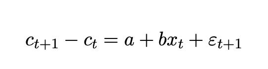
As usual for Bob, it all starts with a simple clever idea. In asset pricing, price is present value of dividends, so price follows a random walk. In the permanent income model, consumption is proportional to the present value of income. So consumption should follow a random walk too. Why not test that hypothesis just as asset pricers were doing in the 1970s, by running regressions,

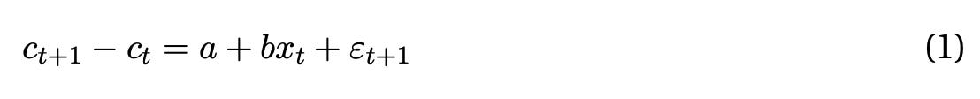
We should see b = 0 for any variable x visible at time t, including past consumption and income. By and large, Bob found that consumption did follow a random walk. The exception, that stock prices slightly forecast consumption growth, might easily be understood with the benefit of hindsight that stock prices reflect variation in expected returns, or that stock prices can more quickly reveal information about future income than the time-averaged consumption data.

Bob's finding became part of the surprising success of 1970s rational expectations in macro and finance. The unwelcome success of the PIH was so controversial at the time, that Bob reports some of the MIT bigwigs semi-seriously talked about revoking his PhD for fraternizing with the enemy. Economics was always ideological, and separated into tribes. However, one can be a little bit nostalgic for macro wars that cared about policy results rather than just methodology.

As usual for Bob, that simple idea ends up having deep consequences. This butterfly did lead to thunderstorms.

2 Background: 1970s Macroeconomics

To understand how Hall changed things, you have to understand where macroeconomics was in the 1970s.

In the late 1970s, economists had begun to formalize the intuitions in Milton Friedman's permanent income hypothesis using the simple linear-quadratic model. If you want to be a macroeconomist, you should know this model by heart. A consumer maximizes

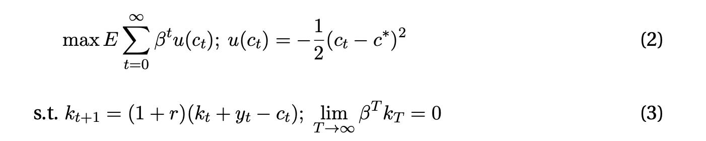
where c= consumption, k= wealth, y= income, and the rest are parameters with β = 1/(1+r).

The first order condition is

Consumption should follow a random walk, which Bob tested by running the forecasting regression (1). As with finance, that economists cannot predict well, usually an insult, is a measure that theory is right.

At the time, though, economists focused on full solutions of the model. Plugging the first order condition into the budget constraint, consumption is proportional to asset wealth and the present value² of future income

Taking innovations and using the first order condition, the change in consumption equals the innovation to the present value of income

This is a nice expression since it leaves out wealth.

We can compute full model solutions. Add an AR(1) model of income, for example

and (5)-(6) become

Now, why did this matter? Much of the profession was in the thrall of ISLM modeling, and Hall was part of the rational expectations revolution that overturned that approach. Typical models looked like

with C= consumption, Y= income K= wealth, I= investment r = interest rate and G= government spending, and U and V are disturbances. One big debate was over the size of the marginal propensity to consume α, and consequently the “multiplier” connecting equilibrium output to government spending. The original permanent income hypothesis (Friedman, 1957) suggested a much smaller marginal propensity to consume out of the transitory income movements that Keynesian stimulus could produce, and hence a smaller multiplier, which is why Bob’s MIT colleagues hated the PIH. Yes, economists are still fighting about marginal propensities and multipliers 72 years later. 

In the late 1970s, this ISLM approach was falling apart due to the “rational expectations” work of Lucas, Hansen, Sargent, Prescott, Sims and others. First, its parameters are not “structural” or “policy invariant” (Lucas, 1976). The “marginal propensity to consume” α is not a feature or preferences or technology, a supply or demand curve. It is a “mongrel” parameter, a combination of the risk free rate and the persistence of income. If the persistence of income ρ changes, (9) shows that the MPC changes too.

Second, and related, Sims (1980) savaged the whole effort. He pointed out that estimates of those models ignored the “cross-equation restriction” linking ρ in (7) to the MPC in (9). More deeply, economics starts with people and businesses, not consumption and investment. People simultaneously decide consumption, saving, labor supply, money demand, limited by their budget constraint. Businesses simultaneously decide investment, output, labor demand, limited by a budget constraint. Governments decide spending, taxing and borrowing limited by a budget constraint. And all these agents decide these questions with an eye to the future. They decide today’s consumption vs future consumption also limited by a budget constraint. An equation describing “consumption” ignores all that. Half a century later, economists still estimate marginal propensities and talk about them as if they are preference parameters that vary across households. Old habits die hard.

Sims also pointed out that identification in such Keynesian models is “incredible.” There is no reason for the right hand variables (Y) to be uncorrelated with disturbances (U), or for any variable to be a valid instrument. There is really no reason to exclude any of the left hand variables from the right hand side of each equation. Without those “exclusion restrictions” or “orthogonality restrictions” all the equations are the same, just solved for a different variable on the left hand side. Game over.

What do we do instead? What do we do instead? Equations (2)-(9) look like a “partial equilibrium” theory of consumption. But interpreting k as the capital stock, they are also the first and simplest complete general equilibrium model of the economy. Since it has analytic solutions and capital, it is a great one to start with. And in the late 1970s the Chicago program was to construct full general equilibrium models, more general versions of (7) - (9), estimate them (find free parameters, r, ρ, c∗) by say maximum likelihood, and test them. Such models display “cross-equation restrictions” which are the “hallmark” of rational expectations models (Hansen and Sargent, 1980) and address the Lucas (1976) critique.

But estimates of the system (7)-(9) found a huge problem. First, using then-standard estimates (which don’t allow for unit roots), the coefficient ρ implied that consumption moved too much, or was “excessively sensitive” to income. Flavin (1981) is a sophisticated version of that test.

Second, and more deeply, (9) has no error term. This isn’t a small problem. Optimal decisions are deterministic functions of the environment. Any test of (7)-(9) in which the consumption function has less than 100% R2 must reject with 100% probability. The model has a “stochastic singularity.”

Third, and fatally, the cross-equation restriction relies centrally on the assumption that people use the income AR(1), and only the AR(1) to forecast future income. It is not enough to “model” income as an AR(1). The time-series model of income has to be exactly the same as people use to forecast their income. If they see any information beyond current income, the model is wrong.

This is a deep and general point that dawned around the time: Any estimate or test must still work if agents in the economy have more information than economists put in our models or estimates. Testable predictions must condition down from people’s information to the economists’ much smaller information. An estimate and test of (7)-(9) violates this requirement.

(Hansen and Sargent, 1980 recognize the agent information problem and the 100% R2 problem, and indeed are one of the pioneers in pointing them out. They may not be the first, but it’s where I learned about it. p. 9 “This paper develops two different models of the error terms in behavioral equations. Both models use versions of the assumption that private agents observe and respond to more data than the econometrician possesses....dynamic economic theory implies that agents’ decision rules are exact (non-stochastic) functions of the information they possess...” In the context of (7)-(9), if agents use some other variable zt as well as yt, or even an additional lag as in an AR(2), then an error term will appear when the econometrician uses the AR(1). However, the properties of such error terms are not comforting for econometricians, including non-invertible moving average representations (p. 18).)

3 Less is More

Finally, it’s time to come back to Hall. The regression (1) which tests the first order condition rather than the full model solution is robust to the possibility that people see more than we do. Thus it shows that such tests are possible.

This shift has huge implications. You cannot estimate, survey, project, or otherwise model future income, discount it back, compute what consumption should be, compare it to actual consumption, and declare a puzzle. People might have more information, and make a different forecast. Hansen, Roberds, and Sargent (1991) formalize this observation in a hard to read but still classic paper. They show how using consumption itself to forecast income can summarize people’s unobserved information, and how to extend just a bit beyond the random walk.

We should write the quadratic utility PIH as

Turning it around, observing consumption on the left reveals to us that slice of the consumer information set.

One can condition down, to conclude

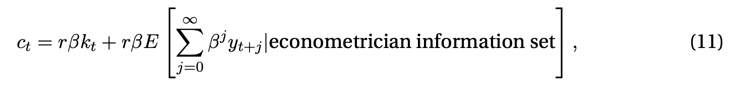
but only if that information set includes consumption. You cannot forecast income with variables that exclude consumption, and then test the relationship.

Finance in the 1970s started to explore the idea that price is the expected discounted present value of future dividends. Like (7)-(9) the natural way to “test” this prediction is to form an estimate of dividends, discount them back, compute the model’s “prediction” for price, and see if it is equal to the actual price. Such estimates fail by huge amounts. But starting in the late 1970s, the similar realization percolated into finance: Such tests assume that agents have no more information than the economist uses to forecast dividends.

The Fama (1970) “joint hypothesis problem,” which became the Harrison and Kreps (1979) and Hansen and Richard (1987) discount factor existence theorem, also doomed tests of the present value relation per se. Absent arbitrage there exists a discount factor so that observed prices equal the present value of dividends. Game over for testing whether price equals the present value of dividends. Nobody has expressed the same idea for the permanent income hypothesis, but it evidently applies as well. So tests of present value relations are twice doomed by unobservables.

You cannot estimate, survey, project, or otherwise model future dividends, coupons, or government surpluses, discount them back, compute what price or value should be, compare them to actual price or value, and declare a puzzle. This limitation has not stopped empirical asset pricing from being incredibly productive. You just have to do other things. As Hall did.

Modern empirical finance, crystallized by Campbell and Shiller (1988) gives up on testing the present value relation, instead treating it as an identity and measuring how much price variation comes from dividend growth and how much from discount rates. Our job moved from test to measurement, from declaring that present values are per se rejected to puzzling just why discount rates account for so much price variation. Campell and Shiller’s measures are robust to the possibility that agents see more information than they include in the VAR. As Hansen Roberds and Sargent recommend, they include the price in the forecasting VAR, which summarizes people’s extra information.

Somewhat frustratingly to a child of the 1980s like myself, the requirement that tests should not assume agents have no extra information is still frequently violated by papers that get published in fancy journals, presented at top conferences, cited and followed with literatures. Have referees, asking for one more robustness test in online appendix D, not heard of these basic theorems? People love to proclaim puzzles, I guess.

Ask of any paper you read, what if agents have more information than is represented in this VAR? Does the test still work if they do? If not, remind them of Hall. (Likewise, ask if the paper violates the existence of a discount factor theorem. Surprisingly many do.) Likewise, “unobserved individual heterogeneity” plagues a lot of microeconomic empirical work. Many regressions assume that they have controlled for everything.

4 Beyond the Random Walk

The random walk / PIH model spawned lots of work, and I do not pretend a comprehensive or fair literature review.

Campbell and Mankiw (1990) interpreted a small coefficient of consumption growth on lagged income as excess sensitivity. That’s based on forecasts, and different than the cross-equation restriction of (7)-(9). Campbell (1987) looked at the issue another way. Under the PIH, saving should forecast labor income. In a time of temporarily high labor income, people save, and then spend when the rainy day comes. Campbell also inaugurated a new sensitivity to the fact that macroeconomic variables have unit roots and a cointegration structure, so it is inappropriate to detrend them. This is a delightful use of consumption, or its inverse, saving, to measure information that agents have which econometricians do not see. Moreover, nothing else that agents can see should help to forecast the present value of labor income. Campbell finds the glass half full: “Saving helps to forecast declines in labor income in all the estimated VARs. But the very tight restrictions of the model are strongly rejected in VAR systems with more than one lag.” (p. 1273.) The latter means that other variables help to forecast the present value of labor income.

One useful (I think) extension is Cochrane (1994) “Permanent and Transitory Components of GNP and Stock Prices.” Cointegration and unit roots followed random walks³ in the 1980s.

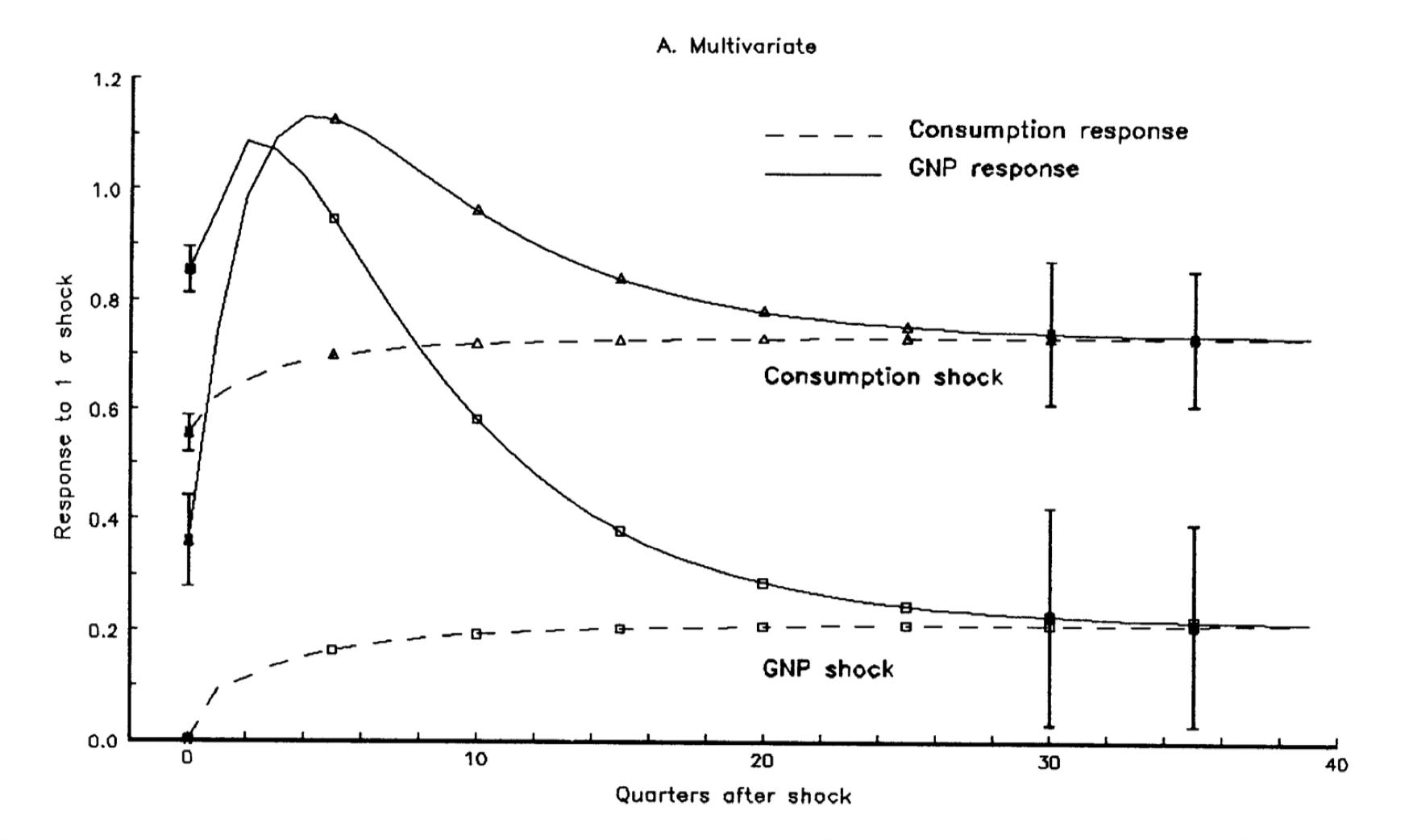
Consumption and income are cointegrated (in logs). They share a trend, but the consumption / income ratio is stationary over time. Thus the ratio of consumption to income must forecast consumption growth or income growth, to bring that ratio back to its mean. Table 1 shows what happens when you forecast consumption and income growth with the consumption/income ratio. Hall’s random walk stays true with this extra forecasting variable. Instead, the consumption/income ratio helps to forecast income.

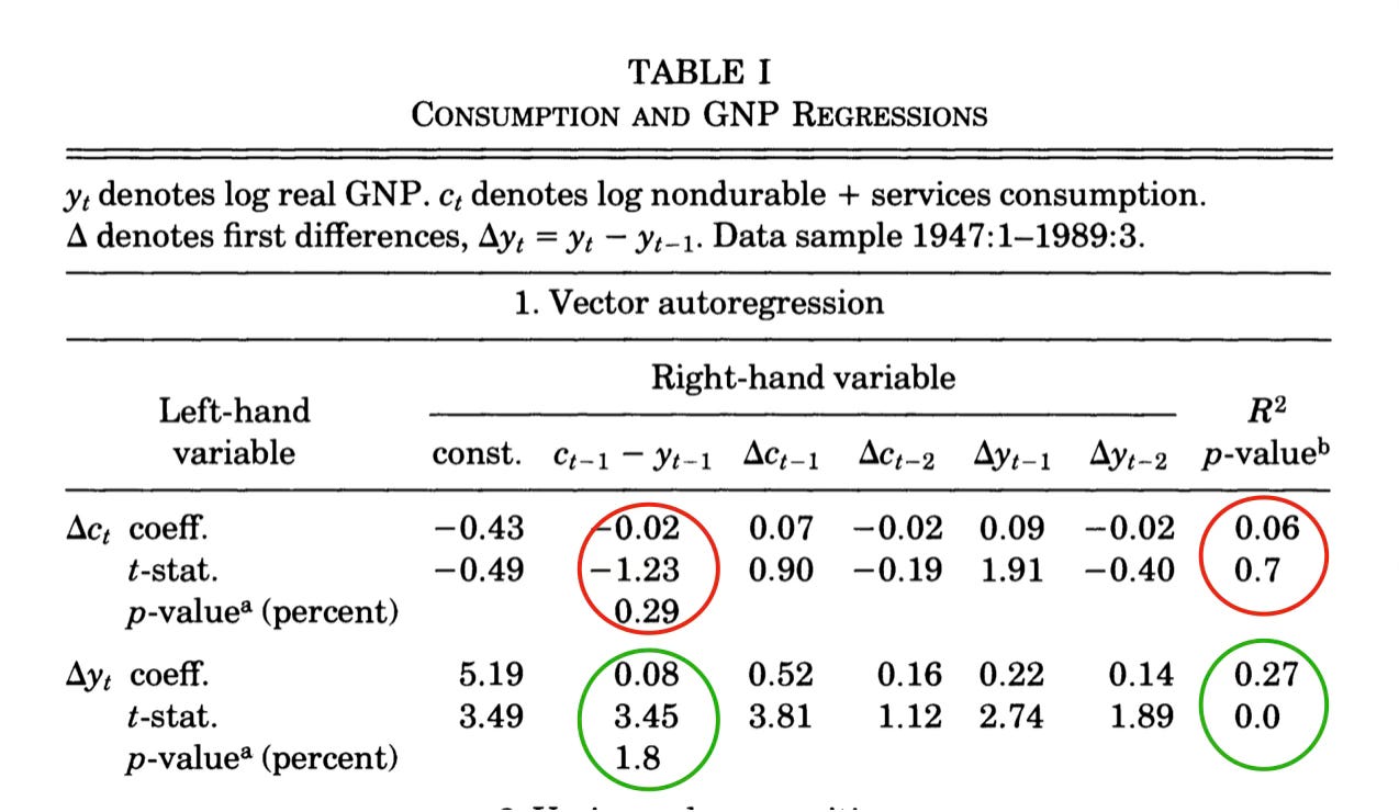
Figure 2 presents the corresponding impulse-response function. Consumption is still a random walk. But a rise in income with no change in consumption is purely temporary. That consumption is (close to) a random walk means that consumption is a good stochastic trend for income. Since the consumption-income ratio is slow moving, it does a much better job of forecasting long-run income than conventional forecasting variables do, even if those might do a better job of forecasting income growth one quarter ahead. Thus consumption is a better measure of the unit root or stationary component of income than anything you can find in past income. Using consumption in this way gives a much better estimate of the random walk or unit root component in income than you can find from income itself. (The question I posed in Cochrane, 1988, “how big is the random walk in GNP?” using univariate methods is much better answered by including consumption.) In the economic interpretation, again, consumption reveals to the macro econometrician consumers’ information about the long-run trend in future income, just as stock prices reveal to the finance econometrician a slice of information that investors have about future stock dividends and returns. Turning the PIH around backwards, to tell us the information in consumption about future income, is as important as its direct use to understand consumption.

Figure 2

5 From Random Walks to GMM

Once we no longer wish for full solutions, especially analytic solutions, there is no reason to specify the rather unrealistic quadratic utility and a constant interest rate. Hall already pointed this out. The prediction

becomes

or with power utility

The Hall regression

becomes the nonlinear regression

The proposition that consumption follows a random walk generalizes to the proposition that marginal utility, discounted by returns, should follow a martingale.

Hansen (1982) showed how to easily run such nonlinear regressions by GMM (Generalized Method of Moments), and Hansen and Singleton (1982, 1983) did it. The results were not as successful as Hall’s random walk, but we’ll get to that in a bit.

This shift marks a second fundamental change sparked by Hall. (The first was recognizing and overcoming the agent information problem.) ISLM models, for all their faults, had one wonderful property: They allowed a division of labor. One economist could work on consumption, one could work on investment, one could work on money demand, and then a team constructing a large scale model could simply put all their work together. If we switch to estimating and testing full general equilibrium models, each author has to specify every part of the model and start over again.

But Hall, and more explicitly Hansen and Singleton, allowed economists again to study preference parameters by themselves, without writing and solving a full general equilibrium model. Other economists could study firm behavior by itself. Then, general equilibrium modelers could again assemble elements from these estimates. Macro could exploit division of labor again. This appreciation in particular came from Bob Lucas.

That program has worked out to some degree, though not as much as one might have hoped, and not as much as in the construction of the first large-scale Keynesian models. Following Hansen and Singleton, economists wrestled with preferences, now to account for asset return data rather than the marginal propensity to consume. The level and time variation of the equity premium – the R part, not the c part of the regression – pose a puzzle leading to innovations such as recursive (Epstein and Zin, 1989) and habit (Campbell and Cochrane, 1999) preferences.

Those preferences have made their way into general equilibrium macro models, though often really because they helped the impulse response functions of those models. The preference studies became places to look for better general equilibrium ingredients. And macro as a whole has still suffered from a lack of division of labor. People introduce one new element in a general equilibrium model, show it helps, and then move on. Few of the new elements stick.

The alternative program was “calibration” as announced and practiced by Kydland and Prescott (1982). In this program, microeconomic empirical work rather than GMM estimation would tell us about preferences and technology, which macro modelers could then incorporate into general equilibrium models. This too would overcome the division of labor problem. Sadly, when macroeconomists actually looked at microeconomic evidence, our belief that surely they all had this figured out and could provide ready estimates proved illusory. Micro empirical work struggles to measure preferences and technology every bit as much or more than macro does. Evenwhen it succeeds, aggregation from micro to macro proves very hard. Aggregation can result in representative agent preferences and technology that look utterly different from underlying microeconomic preferences and technology.

“Calibration” then took on another meaning. Again, full equilibrium models like (7)-(9) display “stochastic singularities,” equations with no error term, and part of Hall’s effect was that economists took notice of this fact. The Q theory of investment likewise says investment = a function of Q, the ratio of stock price to book value, with no error term. You can’t formally estimate and test a model with no error term, as it is immediately rejected. It has zero chance of being a complete description of the data. Adding measurement error or preference shocks is no solution, as then the entire focus of estimation (finding parameters to make the model fit as well as possible) and testing becomes the stochastic structure of the measurement errors or preference shocks, not the fit of the economic part of the model.

The second meaning of “calibration” in Kydland and Prescott (1982) was then to evaluate the model by selected economically relevant moments, such as the relative variance of consumption, investment, and income, while ignoring the 100% R2 implications For example, it is a success that in response to transitory shocks, consumption in real business cycle models follows something like a random walk, with bigger swings in savings and investment as people save for a rainy day and dissave in bad times. (The PIH lives again, and its intuition pervades more complex models.)

Economic models are not potential literal descriptions of reality. Economic models are quantitative parables. Statistical theory starts with the assumption that the model is potentially a literal description of reality. We know that’s false. How do you evaluate a quantitative parable?

Well, you point out the ways in which it organizes whatever seem like intuitive and robust and important features of the data, while recognizing that other features – such as a 100% R2 prediction – are false. Along with this evaluation, “calibration” started to mean selecting parameters by some moments that seem economically relevant for the parameters, and then evaluating (don’t say “testing”) the model by other moments, all relatively disconnected from microeconomic evidence or GMM macro estimates. Sometimes the former are “first” moments such as growth ratios and the latter are “second” moments such as variances, though Hansen long ago warned me against such language as the variance starts with the first moment of a squared variable.

Along the way, however, notice that testing “cross-equation restrictions” epitomized by (7)-(9), once the “hallmark” of rational expectations, have largely faded away. They are typically not robust to agent information.

6 Intertemporal Substitution

My second Bob Hall paper, “Intertemporal Substitution in Consumption,” Hall (1988), dove in to the questions raised by the early Euler equation tests. The latter mostly offered formal rejection without much economic intuition (unless you really know where to look, but most people at the time did not). To recap, the first order condition is, with power utility,

With a risk free rate

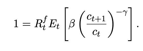
and approximating,

where δ= log(β) and ∆ct+1 = log(ct+1/ct). Therefore, we run a regressio

Consumption should not be a random walk. Consumption growth should be predictable from the real interest rate. But it should only be predictable by the real interest rate. We should see b= 1/γ, a measurement of σ= 1/γ the elasticity of intertemporal substitution, and d= 0.

Bob looked over a variety of estimation methods, and basically came to the conclusion that real interest rates don’t reliably predict consumption growth as they should (my interpretation). Consumption is more of a random walk than it should be! To the extent he was able to measure anything, he found a small intertemporal substitution coefficient, corresponding to an inverse substitution elasticity of about 10. This was a puzzle at the time, but in retrospect lines up with high risk aversion in asset markets. Maybe power utility isn’t so bad after all.

We can parcel out the Euler equation into a risk free rate effect, (12) and a risk premium effect

The Mehra and Prescott (1985) “equity premium puzzle” showed that a very high value of risk aversion γ is necessary to understand the average return difference between stocks and bonds and pointed to the difficulties of the consumption based model in that regard. Hansen and Jagannathan (1991) link that more clearly to the basic first order condition, apart from Mehra and Prescott’s full model. Hall here showed the parallel empirical and economic difficulties in understanding intertemporal substitution. Together they set the path to understanding the failures of Hansen and Singleton’s tests.

The question of intertemporal substitution is as relevant as ever, and Hall’s provocative result that the most important equation in all of macro really doesn’t work remains a thorn in our side.

Figure 3

The first equation of the dominant new-Keynesian model is Hall’s equation, written as

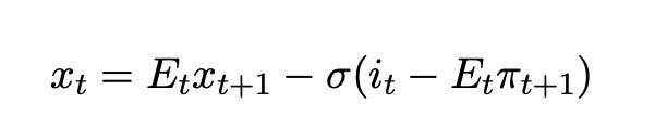
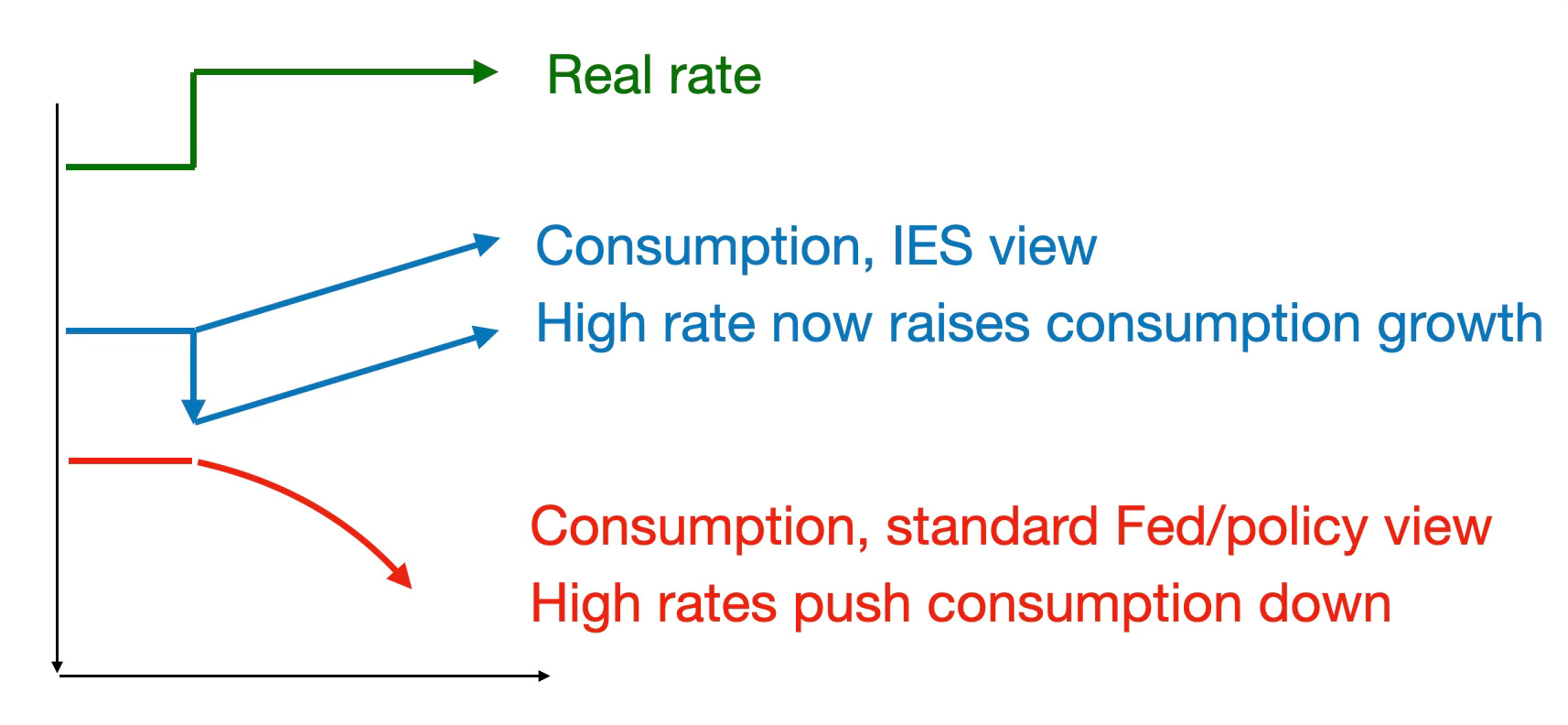
(Here x represents the output gap, equal to consumption in a model without capital.) Higher real interest rates should raise consumption growth going forward. Higher interest rates can only lower consumption at all if consumption jumps down before rising, as illustrated by the blue lines of Figure 3. (Habits can change that relationship, but only by slipping a derivative not by changing a sign. Higher interest rates raise the rate of change of consumption growth.)

40 years later, this basic equation remains quietly controversial. Nobody seems to believe it when talking about policy, but it passes without question when talking about models. The utterly standard policy view is that higher real interest rates lower future consumption and income, as illustrated by the red line in Figure 3. If you write a model in which higher real interest rates lower consumption growth, people will look at you really strangely. If you stand up in a FOMC meeting or write an oped and say that higher real interest rates will raise future consumption and output growth, people will look at you just as strangely. It’s interesting that in academic economics we can repeat things without batting an eyelash that nobody in the policy world believes, while the policy world believes a completely different sign, and economists who go back and forth never notice. Economists can say higher interest rates raise consumption growth yadda yadda in an academic seminar, and then explain how higher interest rates will soften the economy going forward (with long and variable lags), exactly the opposite sign, in policy discussions. Cognitive dissonance reigns.

(To be fair, most policy people will, if pressed, acknowledge that higher real interest rates should go with higher consumption growth, as higher nominal should go with higher inflation, in some suitably far off theoretical long run. But that long run is a long way from policy concerns.)

7 How's it Going?

Especially given the importance of the issue, it seems worth seeing a bit how it's going. In a word, unresolved, but with some interesting possibilities.

The tests of the 1980s glossed over many practical issues. (Hall 1988 actually mentions quite a few of these, unusually.) Consumption is temporally aggregated. It is the average value for the month, quarter or year in question, while asset returns are point to point. Consumption is seasonally adjusted, which introduces a two-sided seven-year moving average. The theory refers to the flow of consumption, not to the purchase of durables which is really an investment. Consumption services data include housing, healthcare, financial services, and insurance, which most people don't adjust at high frequency. Nondurable goods “last generally less than 3 years” per the BLS, not 1 month. We buy a lot of even ``nondurable'' clothing once a year at Christmas. A year seems the minimum time scale at which households reassess their consumption levels. We don't have a good measure of the real interest rate. Rates we have are not that accessible to most households, and perhaps short-term bond rates are contaminated with liquidity premiums.

Given all this, it would be amazing if consumption growth in adjacent months obeyed any of our Euler equations! And 40 years have passed. Perhaps some of Hall's intertemporal substitution problem was simply that real interest rates didn't vary that much. Lately, they have.

I'll show you three glimmers of hope that maybe intertemporal substitution does, at last, work better than it seemed to when Hall wrote. (Again, this is not a comprehensive literature review.)

First, Di Tella, Hébert, Kurlat, and Wang (2023) sought a way to get around potential liquidity premiums in reported nominal rates. They compute a zero-beta rate, the real return on a portfolio of stocks that are uncorrelated with every risk factor one can think of. Then they run forecasting regressions

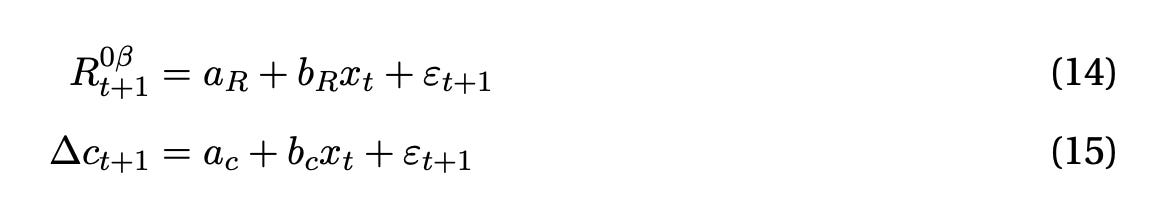
With a list of popular forecasting variables x.

Figure 4. Source: DI Tella et. al. (2024).

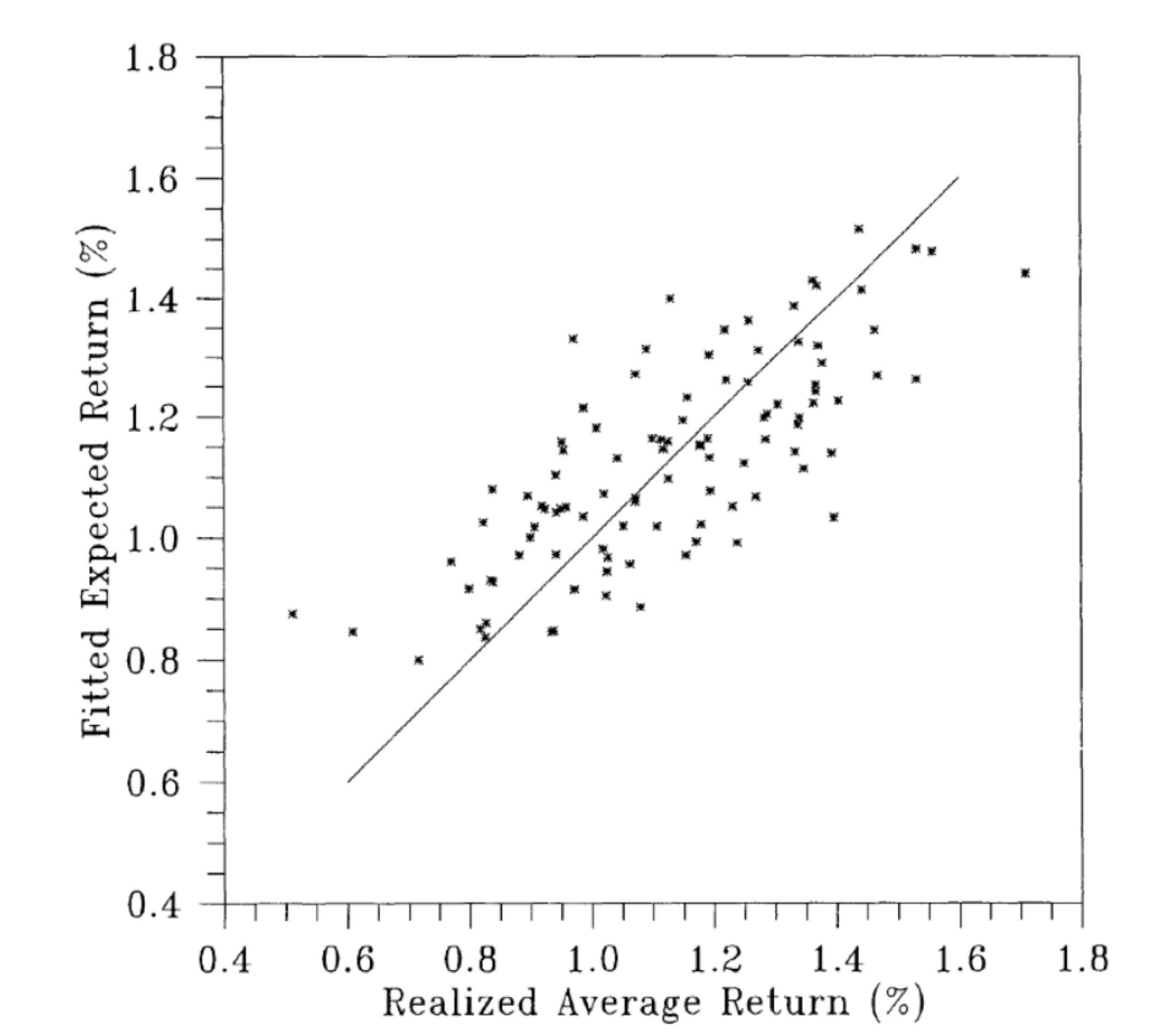
Figure 4 plots the forecasted consumption and zero beta rate, the fitted values of (14)-(15). The correlation is fantastic. Comparing left and right axes, again the implied inverse substitution elasticity is about 10, as Hall found, on the order of standard risk aversion estimates, not the usual value on the order of 1.

Yes, it’s too good to be true in a few dimensions. The plot reflects some overfitting. If there were only one forecasting variable, they two lines would be perfectly correlated. With two or more variables, there is no guarantee that the forecasts will line up, but you’re looking at two different projections on to forecasting variables, not consumption and the interest rate alone. The zero beta rate is a volatile stock portfolio involving long and short positions. The plot uses full-sample estimates, not rolling forecasts. It’s hard to believe that the actual risk free rate varies from -20% to +30%, or that the conditional mean of any stock portfolio has that much variation. But even this much success is remarkable considering Hall’s JPE-worthy catalog of failures.

Figure 5. The consumption CAPM using fourth quarter consumption and the Fama French 25 size and book/market portfolios. Source: Jagannathan and Wang (2007)..

Jagannathan and Wang (2007) notice the durability of much “nondurable” consumption plus time aggregation. As a simple solution, they use fourth quarter to fourth quarter annual data, rather than (say) Hansen and Singleton’s monthly data. They are interested in the equity premium, or the extent to which following (13)

average returns line up with covariances of returns with consumption growth. Figure 5 displays their result, using the Fama French 25 size and value portfolios. Compared to standard implementations of consumption based asset pricing models, just using fourth quarter (Christmas) to fourth quarter consumption creates a decent fit.

Figure 6

To update Hall-style regressions, and inspired by this result, I ran some regressions, presented in Figure 6. I use only nondurable consumption. (Services shows a slightly bigger coefficient on lagged income, but as above services doesn’t really correspond to the kind of quickly adjustable consumption of the theory. Adding habits is an important extension, but I want to follow Hall and I don’t want to write a whole new paper here.) I stop before the pandemic. Consumption is not forecastable at all in the full dataset, but the regression is completely dominated by the huge swings of consumption in the pandemic. (Time series macro will never be the same!)

I forecast fourth quarter to fourth quarter consumption in order to avoid time aggregation, seasonal adjustment smoothing, durability across quarters, and so forth. In single or multiple regressions only the term spread shows a t statistic slightly greater than 2. There remains a point estimate of a little bit of serial correlation in consumption growth, but far below standard significance levels. Lagged income, indicative of “excess sensitivity,” is silent. Remembering that you're not allowed to cherry-pick t statistics, and with an overall R2 of 0.03, I'll summarize the results to say that Hall’s random walk holds up remarkably well.

With log utility, the risk free rate forecast and consumption forecast should be the same. Forecasting the ex-post one-year real return on treasury bills, you see a marked difference. The lagged rate strongly forecasts the current real rate.⁴ Well, interest rates are strongly serially correlated and inflation doesn't noise that up too much.

However, once again with an inverse substitution elasticity of 10, the fdifference between 10 times consumption growth and return is not forecastable! Yes, the consumption growth wasn't significant to start with, so this is a weak result. But consumption growth times 10 does wipe out the interest rate forecastability.

So both versions of Hall remain valid (or at least not overturned by strong evidence.) On its own, consumption looks a lot like a random walk. With a low intertemporal substitution elasticity, the strong forecastability of one year real returns is matched by the barely detectable forecastability of consumption growth.

Hall's results remain valid 40 and 50 years later. But this is extraordinarily weak evidence for the basic question: Does intertemporal substitution work? Do higher interest rates raise consumption growth? It still lies at the heart of all modern macroeconomics.

Part of the problem is that empirical results based on forecastability are delicately sensitive to timing. Whether one variable predicts another one period ahead, or whether consumption growth and returns are correlated enough to justify average returns, are relations that can be destroyed by shifting variables one period forward or backward.

Perhaps more importantly, there is necessarily lots of unpredictable movement in both consumption growth and ex post real interest rates. One can, as I did, fail to reject the hypothesis that consumption growth (times 10 in this case) forecasts and interest rate forecasts move together, but those forecasts are such small parts of actual ex post consumption growth and interest rates that it is hard to see the pattern. That is perfectly consistent with the theory, but makes the theory hard to see.

Retreating from full model solutions to first-order conditions surmounted the agent information problem, but throws out a lot of information that economists might have been able to use to measure and evaluate the theory. I miss those cross-equation restrictions, and estimates and tests based on the 99% of consumption movement that is not forecastable. Shiller (1979), looking at the parallel questions of stock prices, said basically, “Sure, stock prices are not predictable. But you're missing the elephant in the room. Why do they move around so much?” The actual volatility tests morphed into the Campbell and Shiller regressions mentioned above, which focused the question on discount rate variation. Freed from the necessity to formally test models, general equilibrium modelers now work hard to produce models in which stock prices vary (unexpectedly) so much. The real business cycle movement achieved the same thing for consumption, though without this introduction. The RBC statement that consumption is less volatile than income is a full-model statement about ex-post not just ex ante variation. It uses the cross-equation restriction. It just isn’t a "test.”

Figure 7:Growth in real nondurable consumption per capita, and ex post real 1 year treasury rate, 10 year moving average.

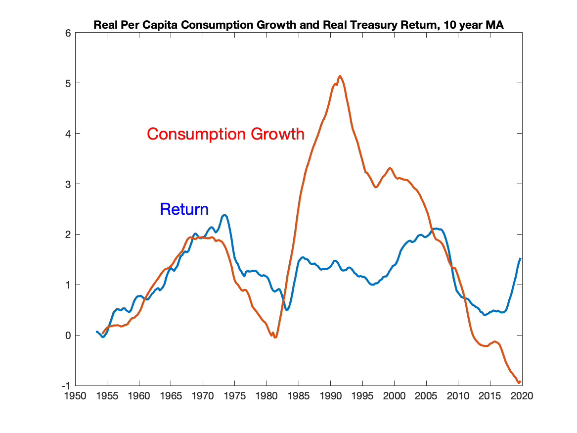
Some direct evidence would still be useful. So, as one indication, Figure 7 plots a 10 year moving average of real per capita nondurable consumption growth, along with a 10 year moving average of the ex-post 1 year real treasury rate. These moving averages elide the timing issues, and smooth out the variation of ex-post consumption and returns. The 10 year moving averages do move together, this time without multiplying by 10.

There is some element of truth in the proposition, quite radical if you think about it, that higher real interest rates correspond to higher consumption growth.

Simple small ideas can have big consequences. Bob always advises to keep some room in your time to pursue such apparently small ideas rather than put them off for years, and you can see some of the wisdom of that advice.

References

Campbell, John Y. 1987. “Does Saving Anticipate Declining Labor Income? An Alternative Test of the Permanent Income Hypothesis.” Econometrica 55 (6):1249–1273. URL http://www.jstor.org/stable/1913556.

Campbell, John Y. and John H. Cochrane. 1999. “By Force of Habit: A Consumption-Based Explanation of Aggregate Stock Market Behavior.” Journal of Political Economy 107:205–251.

Campbell, John Y. and N. Gregory Mankiw. 1990. “Permanent Income, Current Income, and Consumption.” Journal of Business & Economic Statistics 8 (3):265–279. URL https://www.tandfonline.com/doi/abs/10.1080/07350015.1990.10509798.

Campbell, John Y. and Robert J. Shiller. 1987. “Cointegration and Tests of Present Value Models.” Journal of Political Economy 95:1062–1088.

———. 1988. “The Dividend-Price Ratio and Expectations of Future Dividends and Discount Factors.” The Review of Financial Studies 1 (3):195–228.

Cochrane, John H. 1988. “How Big Is the Random Walk in GNP?” Journal of Political Economy 96 (5):893–920.

———. 1994. “Permanent and Transitory Components of GNP and Stock Prices.” The Quarterly Journal of Economics 109 (1):241–265.

Di Tella, Sebastian, Benjamin H´ ebert, Pablo Kurlat, and Qitong Wang. 2023. “The Zero-Beta Rate.” Manuscript.

Epstein, Larry G. and Stanley E. Zin. 1989. “Substitution, Risk Aversion, and the Temporal Behavior of Consumption and Asset Returns: A Theoretical Framework.” Econometrica 57:937–969.

Fama, Eugene F. 1970. “Efficient Capital Markets: A Review of Theory and Empirical Work.” The Journal of Finance 25 (2):383–417.

Flavin, Marjorie A. 1981. “The Adjustment of Consumption to Changing Expectations About Future Income.” Journal of Political Economy 89 (5):974–1009.

Friedman, Milton. 1957. A Theory of the Consumption Function. Princeton, NJ: Princeton University Press. https://www.nber.org/books-and-chapters/theory-consumption-function.

Hall, Robert E. 1978. “Stochastic Implications of the Life Cycle-Permanent Income Hypothesis: Theory and Evidence.” Journal of Political Economy 86 (6):971–987.

———. 1988. “Intertemporal Substitution in Consumption.” Journal of Political Economy 96 (2):339–357. http://www.jstor.org/stable/1833112.

Hansen, Lars Peter. 1982. “Large Sample Properties of Generalized Method of Moments Estimators.” Econometrica 50 (4):1029–1054.

Hansen, Lars Peter and Ravi Jagannathan. 1991. “Implications of Security Market Data for Models of Dynamic Economies.” Journal of Political Economy 99 (2):225–262.

Hansen, Lars Peter and Scott F. Richard. 1987. “The Role of Conditioning Information in Deducing Testable Restrictions Implied by Dynamic Asset Pricing Models.” Econometrica 55 (3):587–613.

Hansen, Lars Peter, William Roberds, and Thomas J. Sargent. 1991. “Implications of Present Value Budget Balance and of Martingale Models of Consumption and Taxes.” In Rational Expectations Econometrics, edited by Lars Peter Hansen and Thomas J. Sargent. London: Westview Press, 121–161.

Hansen, Lars Peter and Thomas J. Sargent. 1980. “Formulating and estimating dynamic linear rational expectations models.” Journal of Economic Dynamics and Control 2:7–46. URL https://www.sciencedirect.com/science/article/pii/0165188980900494.

Hansen, Lars Peter and Kenneth J. Singleton. 1982. “Generalized Instrumental Variables Estimation of Nonlinear Rational Expectations Models.” Econometrica 50 (5):1269–1286. URL http://www.jstor.org/stable/1911873.

———. 1983. “Stochastic Consumption, Risk Aversion, and the Temporal Behavior of Asset Returns.” Journal of Political Economy 91 (2):249–265. URL http://www.jstor.org/stable/1832056.

Harrison, J. Michael and David Kreps. 1979. “Martingales and Arbitrage in Multiperiod Securities Markets.” Journal of Economic Theory 20:381–409.

Jagannathan, Ravi and Yong Wang. 2007. “Lazy Investors, Discretionary Consumption, and the Cross-Section of Stock Returns.” The Journal of Finance 62 (4):1623–1661. URL http://www.jstor.org/stable/4622313.24

Kydland, Finn E. and Edward C. Prescott. 1982. “Time to Build and Aggregate Fluctuations.” Econometrica 50 (6):1345–1370.

Lucas, Robert E. 1976. “Econometric Policy Evaluation: A Critique.” Carnegie-Rochester Conference Series on Public Policy 1:19–46.

Mehra, Rajnish and Edward C. Prescott. 1985. “The equity premium: A puzzle.” Journal of Monetary Economics 15 (2):145–161.

Shiller, Robert J. 1981. “Do Stock Prices Move Too Much to be Justified by Subsequent Changes in Dividends?” American Economic Review 71 (3):421–436.

Sims, Christopher A. 1980. “Macroeconomics and Reality.” Econometrica 48 (1):1–48.

 

1. I thank Tom Engsted and Ed Nelson for helpful comments.

2. Thanks to a comment by David Seltzer, I realize that I (and we) have been using the wrong terminology in the PIH. The present value of the income stream, which is its market value, is its stochastically discounted value

Future consumption and future income are correlated, so this value is not the same thing as the right hand side of the PIH

Don't go too far down this rabbit hole. The quadratic utility PIH allows zero and negative marginal utility which plays havoc with asset prices. But it is not correct to say that consumption depends on the “present value” of future income. I'm not going to try to correct 50 year old terminology!

3. A variable with a unit root (1− L)xt = a(L)εt generalizes a random walk (1− L)xt = εt. Two variables are cointegrated if they each follow unit root processes but a linear combination xt + ayt is stationary.

4. I use the December t bond yield minus December t-1 to December t inflation as a forecast variable. I use the December t bond yield minus December t to December t+1 inflation as the real rate to be forecast. The forecasting variable should have lots of information. Since we don't observe a real rate, it does not have to be the actual real rate. The left hand variable does have to be a real return. The question is whether any variable x forecasts the real return, not whether the lagged ex-post real return does so.