Two New Papers

It is still thrilling when a paper is finally published. And I am particularly proud of these two. I also write as Elsevier offers free downloads for 50 days. If you want one, get it now! Here they are:

Inflation Dynamics with a Generalized Lucas Phillips Curve

New-Keynesian Inflation Control is Equilibrium Selection

The question: How do central banks lower inflation by raising interest rates? Or can they? In particular, how can a central bank lower inflation all alone — without coincident tighter fiscal policy? (“Active” or “passive”.) And how can today’s interest rate lower future inflation?

I’m looking for the simplest, explainable, understandable benchmark model of inflation and interest rates (and maybe a bit of output), not a big calibrated black box.

In light of this year’s Nobels, this is also a good time to comment. Though the basic new Keynesian model dates from the 1990s and Mike Woodford’s book was published in 2003, there is plenty to do following up on these basic ideas as you’ll see.

Equilibrium selection

You might say, “Duh, the standard three-equation new-Keynesian model answers that question.” “Equilibrium selection” puts together exactly why that isn’t the case.

The model is the standard IS (intertemporal substitution) and Phillips curve,

with x = output, i = nominal interest rate, pi = inflation, r is the steady state real rate, and sigma and kappa are parameters. This is the continuous-time version of the more familiar

I leave out the expectations to study the response to a shock. I’m going to completely follow the NK philosophy here; no fiscal theory funny business.

Eliminating output and solving the second-order differential equation for inflation, the solutions are

Inflation is a two-sided moving average of the nominal interest rate, with positive coefficients. Higher interest rates on their own raise inflation. There is also an exponentially-decaying transient, indexed by the constant C or by initial inflation. The NK model needs to add something else, not just the path of interest rates, to fully determine what happens to inflation. The different possibilities are “multiple equilibria” so we need an “equilibrium selection” policy in addition to an interest-rate policy. And the only way to get inflation to decline at all in the presence of higher nominal interest rates is to choose a lower C. Inflation control comes from equilibrium selection. And not from higher rates.

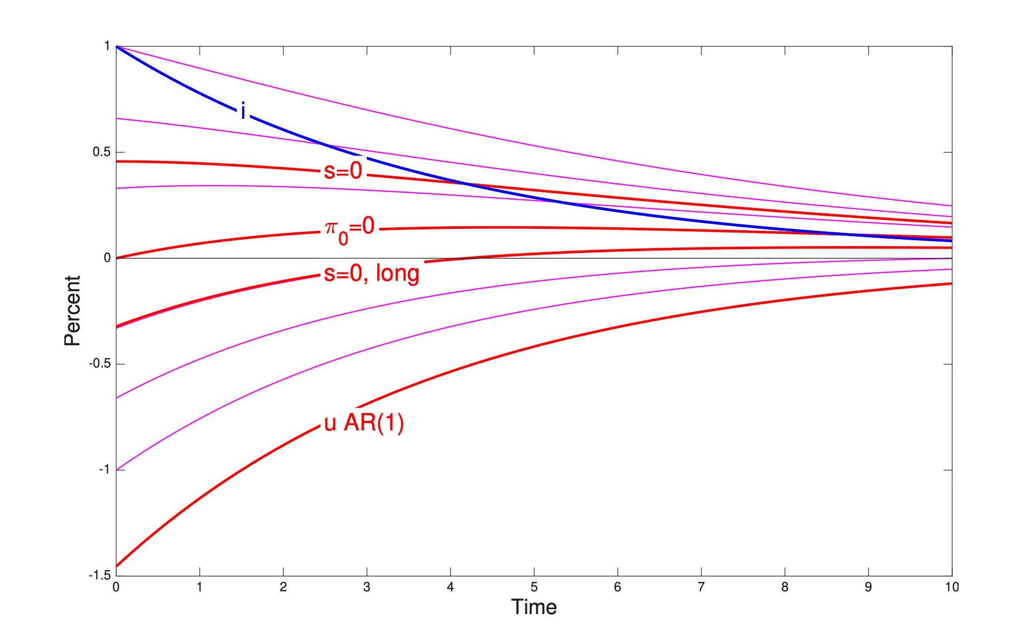
Here is a graph. I suppose the Fed raises interest rates, with a pattern following the blue line. (This is an AR(1), or exponential decay.) Then inflation follows one of these paths, corresponding to different values of C or inflation at time 0. Only the choices with a negative downward inflation jump at time 0 show any decline in inflation at all.

The conventional calculation picks the “u AR(1)” equilibrium. To get that result, you add a Taylor rule for the interest rate

and you specify that the disturbance ut follows an AR(1). Then any but the indicated equilibrium blows up. The Fed selects equilibria by threatening to blow up the economy.

But even granting this blow-up threat, it turns out that there are lots of Taylor rule disturbances ut that produce exactly the same path of interest rates, but produce different inflation paths. They are easy to reverse-engineer: Pick any equilibrium in the first graph, compute ut = it - phi pit, and you have a Taylor rule disturbance that produces the same interest rate path but a different inflation path. These generically follow AR(2), or the sum of two AR(1), the sum of two exponential paths.

So, this standard NK model also makes two, separate specifications of monetary policy: The interest rate follows the path shown in blue, and the Taylor rule disturbance is an AR(1). If we allow AR(2) disturbances, all of the other lines are possible while producing the same path of interest rates. Inflation control is still equilibrium selection. It’s just a lot more buried than following my equivalent approach.

In the standard specification, fiscal policy adapts “passively.” Notice the long period of interest rates above inflation. Interest costs of the debt are high. Who pays those? Fiscal policy must raise taxes or cut spending. So the “equilibrium selection” policy also has a fiscal consequence.

The fiscal theorist, of course, views it the other way around: Fiscal policy “selects equilibria,” or, better, completes the specification of the government policies that determine inflation. You need both the interest rate path and the change (or not) in surpluses to determine inflation.

But you don’t have to take a stand on FTPL. Even with a pure passive fiscal approach, the fiscal tightening must happen. This is not a pure monetary policy change. It is a monetary and fiscal policy change, and the equilibrium selection + fiscal tightening is doing all the work of lowering inflation.

These days, I think it’s important to ask “what if Congress refuses?” And for economic understanding it’s important to ask what is really the effect of interest rates, separate from the effect of Fed-induced fiscal tightening.

The red line marked “s=0” plots an equilibrium that does not require any fiscal change. You could phrase this as a constraint on the time-series process of the Taylor rule disturbance that the Fed may choose, among those that produce the given intrest rate path. You can see that the period of interest rate above inflation is matched by a period of interest rate below inflation, so interest costs net out to zero. And inflation rises throughout. An interest rate rise without fiscal support raises inflation.

This proposition holds more generally. In “expectations and the neutrality of interest rates” I show that even in an old-Keynesian adaptive expectations model, that otherwise well captures standard doctrines, higher interest rates cannot durably lower inflation without a fiscal tightening to pay interest costs on the debt. Intuitively, in that model, higher real interest rates drive inflation down and lower real interest rates raise inflation. So, if the Fed drives inflation down with higher rates, the stock of debt rises due to interest costs. If fiscal policy does not tighten to pay the interest costs or the resulting debt, the Fed must then lower real interest rates for a while to lower interest costs and bring down the debt. That brings inflation right back up again. Let’s call it unpleasant Keynesian arithmetic. Without fiscal tightening, the Fed can only lower inflation at the cost of higher inflation later.

There is a way out, marked “s=0, long.” If I add long-term debt, then the “stepping on a rake” or “unpleasant interest rate arithmetic” mechanism kicks in. Now a persistently higher interest rate lowers long-term bond prices. Since surpluses have not changed (by assumption), that’s a deflationary force. Now we can get the initial jump down in inflation without asking Congress do to anything. And now there is a reason for central banks to raise interest rates. Otherwise, they get even lower inflation with the equilibrium selection policy alone, as higher interest rates raise inflation.

This is the best I have been able to do to produce lower inflation from an interest rate rise without a simultaneous fiscal tightening in the standard new-Keynesian economic framework. I encourage you to find some better simple mechanism that achieves a similar result.

But the resulting model has nothing to do with the standard old-Keynesian intuition, that higher real rates lower aggregate demand, which lowers employment and through the Phillips curve lowers inflation, all going forward. Inflation only goes down from equilibrium selection/fiscal policy. You can see all of this even more clearly in the flexible price model with just interest rate = expected inflation. (See the paper.)

New Keynesian inflation control is equilibrium selection. This is just a fact about the model, and not criticism. This is the model we have. Let’s see how it works, and how to make it work better. The only thing to be critical about is the continued habit of plastering old-Keynesian ISLM intuition, introductions, conclusions, policy implications, and executive summaries on these equations. I tell the joke that new-Keynesians went hunting for a horse — microfoundations of ISLM. They came back with a zebra, and naturally said “look at our fine horse.” Well, that was ok for a while, but now we know that we have a zebra. Celebrate its novelty and let’s see how it works, but stop pretending it is micro-foundations for a horse.

We have made some progress. But inflation still jumps down on the day of the interstate-rate rise. We would like to find a model in which higher interest rates lower inflation going forward. And we would like a simple, robust, and explainable model. Simply saying “prices can’t change for a year,” and adding a smorgasbord of other frictions is unsatisfactory for such a basic idea. Do we really want to say that inflation naturally would jump down and then rise absent some smorgasbord of frictions? Simply alluding to '“long and variable lags” doesn’t work. In today’s macro, dynamics must come from the model.

Generalized Lucas Phillips curve

That brings me to the second of the two papers. Equilibrium selection is, honestly, not that novel. I’ve made the point scattered around many writings before, and I’m getting to be like the stereotype American tourist, who, when locals don’t understand him, just shouts louder. I think I did express it a lot better and all in one place, so maybe this time it will catch on.

The “Generalized Lucas Phillips curve” goes after the central problem of how to get an interest rate rise to lower inflation going forward. Here, I build on the analysis of “Expectations and the neutrality of interest rates.” Standard old-Keyensian (and Friedman 1968 monetarist) adaptive expectations models are unstable. Higher interest rates set off a deflation spiral. That’s how higher rates lower inflation going forward. Rational expectations new-Keynesian models are stable and long-run neutral. Higher interest rates must eventually raise inflation. And we saw above that stability kicks in right away. You can only get lower inflation by an instant downward jump, but then the Fisherian attraction of higher rates starts immediately. But perhaps we can have a model that is unstable in the short run — higher interest rates set off a deflation spiral — but reverts to the stability and neutrality that rational expectations demands in the long run? There is:

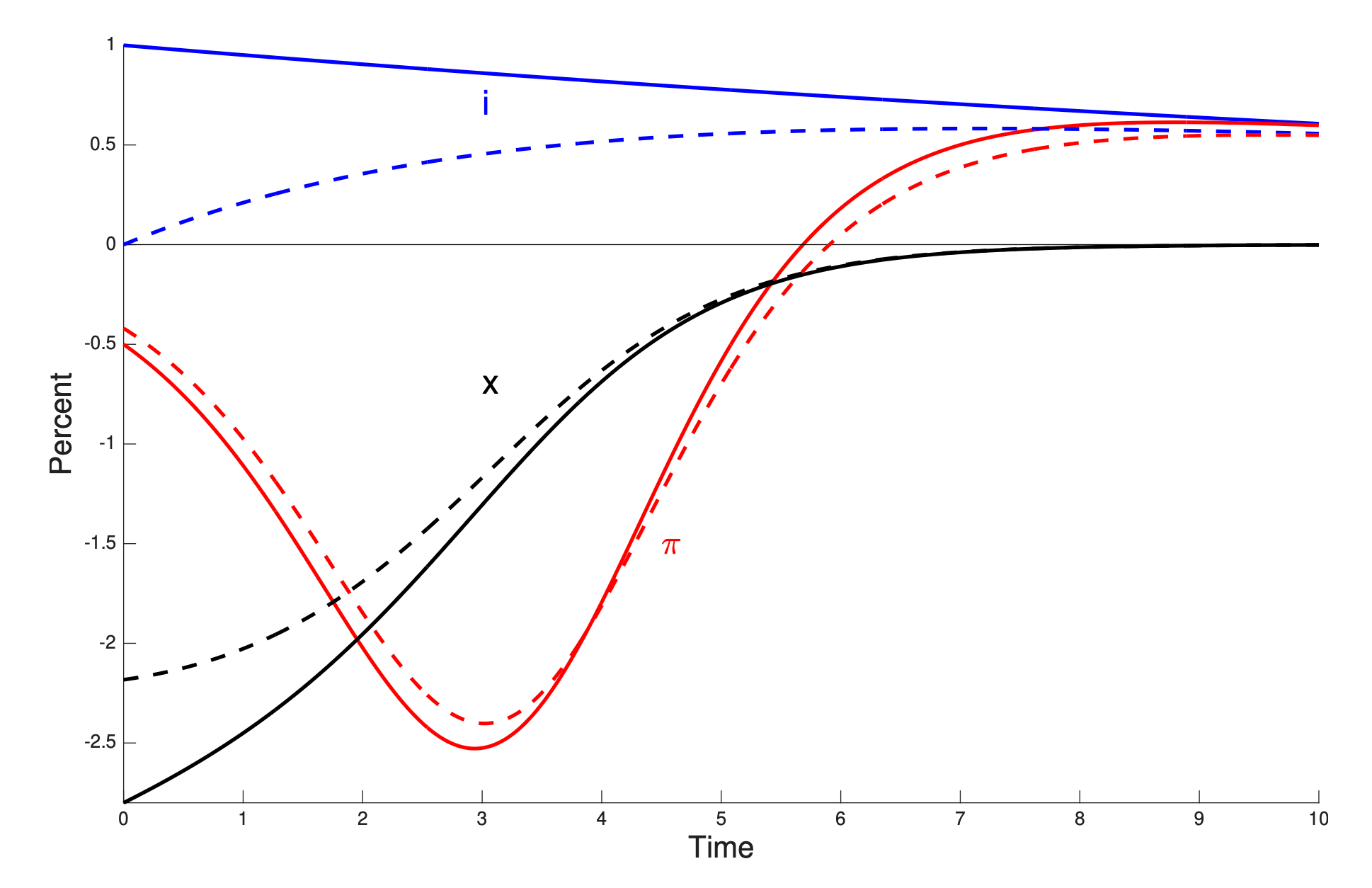
This is the best graph in the paper. Surpluses are constant — this is the counterpart of the “s=0,long” graph above. Start with the solid lines. The interest rate rises persistently, following the usual AR(1) pattern. There is still a small downward jump in inflation, due to the long-term debt mechanism. But then inflation is initially unstable. The initial jump downward gets amplified. It looks old-Keyenesian. After a while, however, new-Keynesian rational expectations take over, and inflation is stable and neutral. That may surprise observers, but most practical people have not seen a lot of long runs where the Fed doesn’t keep moving interest rates around and Congress doesn’t move fiscal policy around.

The model is very simple. I replaced the above Phillips curve with a version of Bob Lucas’ curve,

pt is today’s price level. Output is higher when firms are surprised by inflation, but each firm learns the aggregate price level with a different lag. Alphaj is the number of firms that learn the aggregate with a j period lag. It’s an obvious generalization of Lucas’ curve

I didn’t know this would lead to instability followed by stability. I noticed in “expectations and the neutrality of interest rates” that macro has just basically pushed the index of inflation expectations forward. Adaptive expectations references the Phillips curve to past inflation. New Keynesian economics references the Phillips curve to expected future inflation. How about unexpected current inflation? Might that give the best of both? It turned out to do so. I got lucky.

So the model is just the standard intertemporal IS curve, plus this slightly generalized Lucas Phillips curve. Another plus: It’s trivially easy to solve. I won’t belabor a blog post with it, but the analytic solutions are even easier than the second order differential equation I solved above for the standard NK model. The idea is quite similar to Mankiw and Reis’ “sticky information” Phillips curve, but that one was much harder to solve.

The dashed lines are even better. Again, the long-term debt mechanism still underlies this response, by giving the initial downward jump without a tighter fiscal policy. The key of that mechanism is lowering long-term bond prices. So expectations of future interest rates are the central deflationary force, not the current interest rate. The dashed lines follow a different interest rate policy, an announcement of a future tightening. This has the same deflationary effect, though interest rates do not rise at all in the short run.

This is an important observation for several reasons. Central banks don’t usually raise rates and then let them fall away, like the standard AR(1) exercise. (Maybe that’s been bothering you all along. It should.) Central banks wishing to control inflation usually start on a protracted tightening cycle, like the one in the dashed lines. But in the standard calculation, with the usual Phillips curve and a Taylor rule, such persistent interest rate rises choose an equilibrium in which inflation goes up right away.

Central banks also follow a lot of “forward guidance” — or at least they used to. The standard NK analysis of forward guidance is a bit looney — it says promises further in the future have larger effects today. This is an alternative in which forward guidance is important.

We plot the AR(1) interest-rate exercise because it’s easy, and also because the tiny shocks that “identified” VARs isolate seem to fall away quickly with that pattern. They also seem to have very little effect on inflation. We don’t measure the protracted tightening cycles that we see in history via VARs because those movements are usually responses to other events, like galloping inflation, and hence not “exogenous.” This is a classic case that the “exogenous” identified shock does not isolate the relevant policy question.

This is the best I can do so far, to produce a simple, transparent, easy to solve, baseline model in which higher interest rates lower inflation without fiscal help. It could (and I think should!) take over from the standard Calvo Phillips curve. (Nobody ever accused me of intellectual modesty!)

The paper takes on a lot of the what ifs and what about that are surely troubling you. Habits produce a hump shape in output, but no hump shape in prices. Lagged inflation in the Phillips curve doesn’t work either.

I wish for a better mechanism than long-term debt. Perhaps the next place to look is the IS curve. Interest rates work through capital, investment, and housing, perhaps better than through the usual first order condition. I wish for empirical analysis of the long-term debt mechanism. (I don’t know how to find shocks orthogonal to fiscal policy, reasonably exogenous, and giving rise to persistent interest rate movements. Maybe we have to move past VARs.)

Also, I hold surpluses constant because I think that’s the intellectually interesting question to ask of monetary policy —what can it do alone? If you want to analyze policy and forecast its effects, you should include endogenous surpluses, both from economic effects (more GDP, more tax revenue) and political effects (Gongress does respond to interest costs on the debt). But you should also recognize, as NK economics did not for a long time, when the entire effect is coming from induced fiscal policy and the higher interest rates are, on their own, counterproductive!

There is lots to do! The basic IS/Phillips structure is up for revision, now that we understand the weaknesses of the three equation model and we can handle the fiscal underpinnings of monetary policy. This post is in the end suggestions for future research.