The Fed and risk premiums
It is an article of faith on Wall Street, and in much of the press, that when the Fed lowers interest rates, it sparks a “reach for yield,” a “bubble,” a decline in the risk premium of other assets including stocks and houses. Not so, says a recent excellent paper, “Movements in Yields, not the Equity Premium: Bernanke-Kuttner Redux” by Stefan Nagel and Zhengyang Xu.
(I saw the paper at the recent NBER Asset Pricing Program meeting, along with a great discussion by Annette-Vissing Jorgensen. There were many good papers at the meeting.)
Here’s the issue. When the Fed lowers interest rates, bond prices rise. To the extent that stocks are like bonds, stock prices should rise as well. When interest rates fall, the expected return of stocks should fall. In the Wall Street view, however, stock prices rise more than comparable bonds, and stock expected returns fall by more than interest rates.
The expected return on stocks has two components, the risk-free interest rate plus the risk premium. The risk premium is how much extra return stocks must promise to compensate for risk. In the Wall Street View, lower interest rates spark risk-taking by investors, and lowers the risk premium part as well as the interest rate part.
Economics is a bit more skeptical. Borrowing at 1% to invest in stocks that pay a 4% expected return is the same as borrowing at 6% to invest in stocks that pay a 9% expected return. The expected return of the long-short strategy is exactly the same in either case. Why should the level of the risk free rate matter at all to the spread between stocks and the risk free rate?
Well, frictions, you say. It’s easier to borrow when rates are 1% not 6%. Why? I’m not sure. But it is not one of those obvious parts of economics. It takes some sort of frictions. Economics naturally separates the risk free rate, the price of money over time, and the risk premium, how much you earn for risk.
We can put the same observation in terms of stock prices. For blog post discussion, remember the simple Gordon growth formula, p = d/[E(r)-g] where p is stock price, d is dividend, E(r) is the expected return, and g is the expected dividend growth rate. In turn E(r) = rf + rp, risk free rate + risk premium. So, p = d/[rf+rp-g], price equals dividend divided by risk free rate plus risk premium less dividend growth rate. Now if the Fed lowers the risk free rate rf, stock prices do go up. But the Wall Street view, rp goes down with rf and stocks go up even more.
In sum, it’s perfectly natural that lower interest rates lower stock expected returns and raise stock prices. The question is, how much. Is there a “risk premium” effect in addition to the “interest rate” effect?
Enter Nagel and Xu. The paper is lovely by its very clean measures. Obviously my illustrative formula p = d/[rf+rp-g] will not do. How do we do it right?
One of their calculations uses the Campbell-Shiller decomposition. This formula expresses a stock as the expected value of dividends, discounted by the stock’s expected return. It’s basically the formula I used above, p = d/[rf+rp-g], but with the whole stream of expected future interest rates rf risk premiums rp and dividends, and using forward rates (the rate you can lock in today to borrow from year 9 to year 10 in the future) to measure the rf interest rate part of the stock discount factor. (There is also a beautiful decomposition using dividend strips, but I’ll leave that for the paper.)
Here’s the central table:
You’re looking at regressions. In the first column, the left hand variable is the change in stock price, and in the second column it’s how much the stock price would change, based only on the change in interest rates (forward rates, moving rf only in p = d/[rf+rp-g]), all measured on the day of an FOMC announcement. The two right hand variables, POLICY and FFR are measures of how much the Federal Funds rate moved on the announcement, unexpectedly, i.e. the “monetary policy shock.”
The first row is the most stunning result. Stock prices go down 25.25 bps in response to a 1 standard deviation (about 4 bp) unexpected federal funds rate rise. The bond effect, how much stocks should have gone down based only on the change in long-term interest rates, without a change in risk premiums, is almost exactly the same, 25.66 bp. Interest rates account for the entire effect of monetary policy on stock prices.
Using the FF measure in the second row is not quite as strong. The bond effect is 13.07 and the total effect is 19.89. The t statistic for the difference, in the right column is not significant however. Likewise the calculation using a shorter sample and dividend strips, panel A that I don’t show, isn’t quite as strong.
Annette Vissing-Jorgensen pointed out the puzzling low R2 in the regressions. Apparently, monetary policy shocks account for a trivial proportion of stock and interest rate movements on policy announcement days. What else is moving stock, and especially bond markets so much? I’m a little puzzled also, as when I last looked at high frequency data, it seemed that at least in the window around Fed announcements those accounted for essentially all bond price movements. The low R2 also accounts for the low t statistics.
But point estimates are what matters, and the best guess in this nice paper is simple:
The bulk of the stock market reaction in FOMC announcement windows is explained by changes in the default-free term structure of yields, without equity premium effects.
The previous famous result on this question, by Bernanke and Kuttner, came to the opposite conclusion. Nagel and Xu explain the difference. By using a VAR, Bernanke and Kuttner use how all stock price changes represent risk premiums (a lot) and interest rates (not so much) to estimate that decomposition on announcement days. But Fed shocks may be different from the shocks that move asset prices on other days.
Update:
One can quibble, of course. A correspondent points out that the assumptions required to extend expected dividends to an infinite horizon are assumptions.
One weakness, I think, is the whole monetary policy shock business. That’s not unique to this paper, of course, and one should usually not innovate on multiple dimensions at once.
Their measure of “monetary policy shock” is essentially the funds rate after the meeting minus a measure of its expectation, for example Fed funds futures. Now, on most meetings, especially in the zero bound era, the Fed does nothing. So there is a “monetary policy shock” because a measure of expectations is, typically, 8 bps different from the current and subsequent funds rate, but the Fed does nothing. Is the stock market and bond market move on that day really “the effect of a monetary policy shock?” Romer and Romer’s narrative approach finds no monetary policy shocks at all from 1988 until 2022!
This observation might account for the puzzlingly low R2. If most of the right hand variable is noise, the R2 is low. I would find it’s interesting to look at days that the Fed actually changes the funds rate, and also the days that it changes the funds rate in a substantially unexpected way. As background, Monika Piazzesi and I long ago looked at high frequency data around target changes.
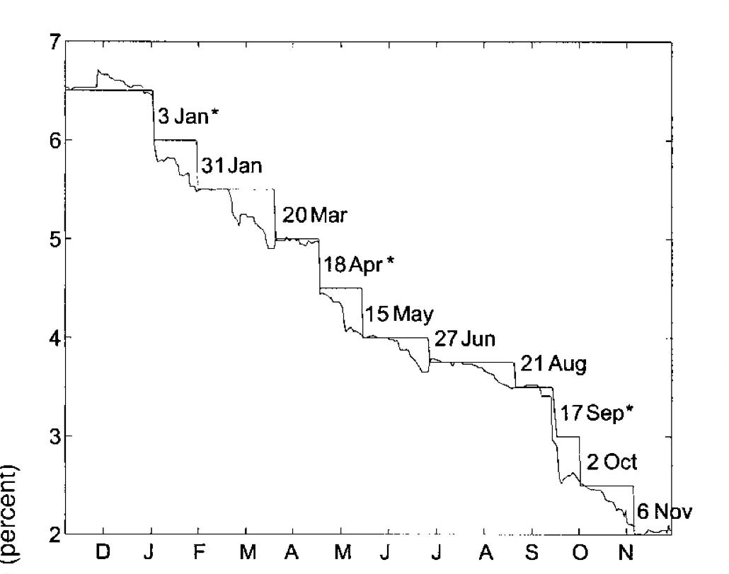
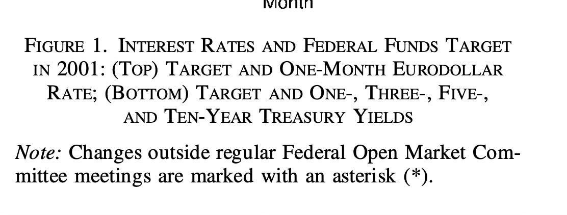
You can see that the one month eurodollar almost perfectly anticipated the scheduled changes. But not exactly. The technique of this, and most other papers on the subject, would find 8 bps “monetary policy shocks” here, and also days that the Fed does nothing. The unscheduled meetings caught markets by surprise. Events like that might be a lot more informative.


I like posts like these.
The correlation between bond and equity risk premia was negative during the Nagel & Xu sample from 1995 to 2022. The consensus of the existing literature is that it was positive in the pre-1995 sample. (Of course, the Fed only began providing after-meeting decision statements in 1994.) Also, we know that the results of the Campbell-Shiller decomposition are very sensitive to the predictor variables included in the VAR. Are the predictors the same as in Bernanke-Kuttner? And why don’t Nagel & Xu use the orthogonalized monetary policy surprises from Bauer & Swanson? You should be able to do this starting in 1988. (See Table 3 here: https://www.michaeldbauer.com/files/mps.pdf. The R2 is about 30%.)
Finally, Cieslak and McMahon have a recent paper that resolves some of inconsistencies you mentioned by looking at forward guidance and the effect on risk premia in intermeeting periods: https://papers.ssrn.com/sol3/papers.cfm?abstract_id=4560220.