Supply Shocks and Nominal Anchors

Updating “Inflation,” I took “supply” and “demand” shocks more seriously, in a FTPL framework. The May inflation surge may make these thoughts extra relevant. (I thank a few thoughtful correspondents, and especially Greg Kaplan.)

Take a stock New-Keynesian model, adding FTPL with short-term debt. The model is an IS curve with a “demand” shock, a Calvo Phillips curve with a “supply” shock, an interest rate rule, and unexpected inflation = the revision in present value of future surpluses. With sticky prices, the real interest rate can vary. Interest costs on the debt can vary, and the present value of surpluses is lower when real interest rates are higher.

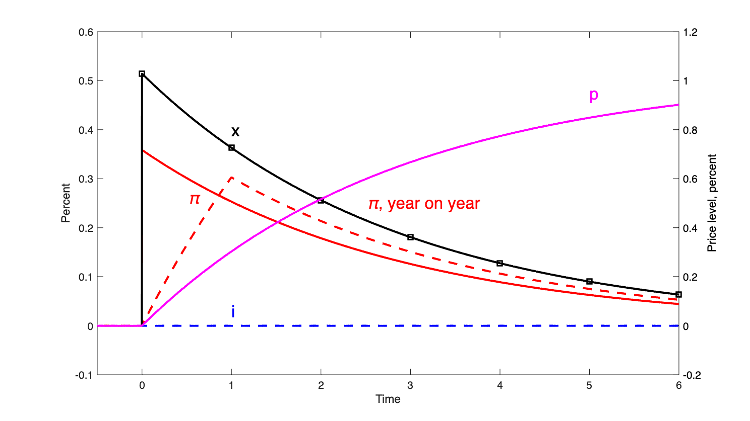
Here is the response of that model to an unfunded fiscal expansion—a decline in surpluses—with no change in interest rate. Inflation surges, but then goes away. In the long run the price level rises. Bondholders lose by a period of low real interest rates — inflation above the nominal rate. In the short run the present value relation B/P = present value of s holds, though B and P have not changed, because the lower real interest rate balances the lower surpluses s. Output surges, following the Phillips curve.

That’s old news. The supply shock:

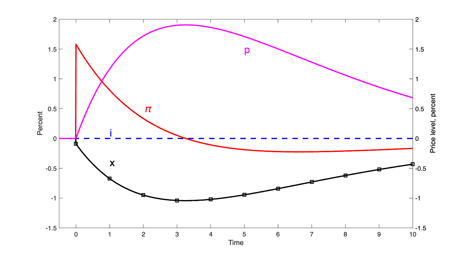
This is an AR(1) shock to the Phillips curve, with no change in interest rate and no change in surplus — no change in monetary or fiscal policy. A “supply” shock is really just an inflation shock. Inflation = expected inflation + (constant) times output + shock. So, no surprise, inflation surges. Output declines. It’s a stagflationary shock, and we move away from the Philips curve.

Here is a “demand” shock to the IS curve, again with no change in monetary (interest rate) or fiscal (surplus) policy

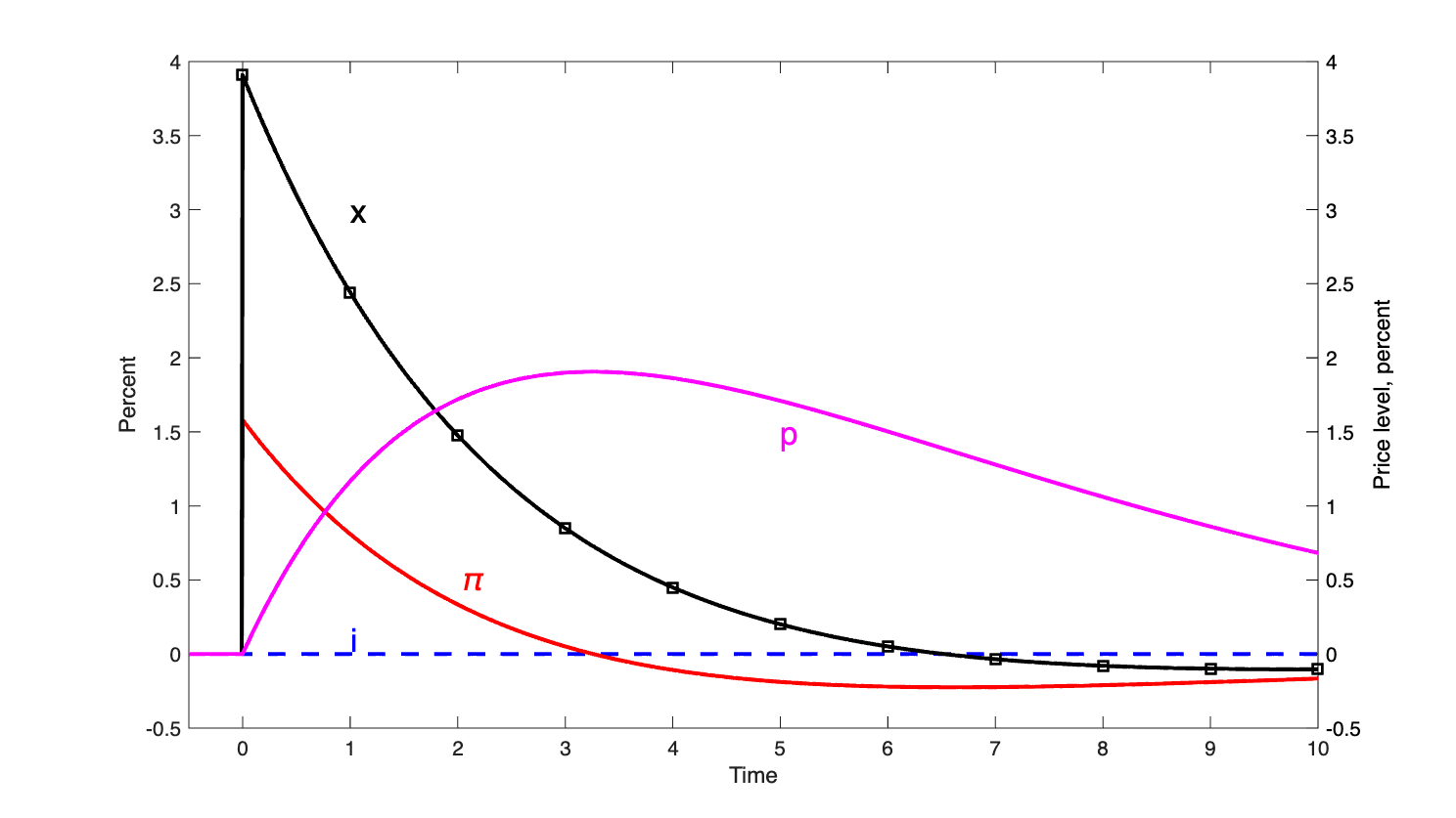
The inflation is exactly the same. This time, following the Phillips curve, inflation produces a strong output response as it did in response to the fiscal shock.

A lot of papers invert the model solution to find which shocks caused inflation in 2021-2022. As you can see, since the inflation pattern is broadly similar, that hinges on the joint behavior of output and inflation. I won’t delve in to that issue here.

Nominal anchors

What about the nominal anchor? When people say “supply” or “demand” (or “greed” or “monopoly” or “price-gouging”) cased inflation, I, like many economists, respond: Don’t confuse relative prices with the price level. The price level always in the end comes from monetary or fiscal policy. But here we have “supply” and “demand” shocks moving inflation, though there is explicitly no change in monetary or fiscal policy.

You can see a big difference in the fiscal shock vs. the supply and demand shocks: only the fiscal shock permanently changes the price level. Not shown, higher interest rates also raise the price level in the long run. So it seems that the nominal anchor is a weak force, that applies in the long run. Supply, demand, and other relative-price shocks can move inflation around in the short run. Maybe inflation is, for a while, just the sum of price changes. When A raises a price, maybe it takes a while for money supply or fiscal theory to drag B’s price down.

That’s tempting, but it’s false. Remember discount rates. With sticky prices, the real interest rate or discount rate part of the present value formula changes. Higher discount rates, or higher interest costs on the debt, lower the present value of surpluses and raise the price level.

Look for example at the response to the demand shock. The period of negative real interest rates (inflation above nominal rate) is initially balanced by the later period of positive real interest rates. There is, initially, no change to the present value of surpluses and no change to the price level. Later, some of the period of negative real interest rates has passed. Now higher real interest rates dominate the present value. The (still unchanged) surpluses are discounted at a higher rate. The price level is higher. Real interest rates eventually revert, so the present value and the price level eventually go back to where it started.

So the price level is always controlled by the nominal anchor, even in these simulations. Real and relative-price shocks do not of themselves change inflation. We don’t go back to thinking of inflation as just the sum of price and wage decisions. But the nominal anchor is the discounted value of surpluses, not surpluses themselves. Other shocks, by inducing changes in the real rate of interest, induce changes in the nominal anchor. Monetary and fiscal policy would have to actively offset those changes if they wished to produce a steady price level.

You could still view the undiscounted nominal anchor as a long-run attractor. The discount rate soaks up other shocks so that the present value relation still holds. In that way you could still think of supply and demand shocks themselves causing inflation, and the real interest rate just soaking up variation so that the present value relation holds. But equalities are equalities and it’s dangerous to think about which one causes which, which equation is stronger than another, and which direction causality runs.

The importance of discount rate variation in the present value formula in all of thse responses offers a good reason why fiscal theory is not immediately noticeable to practical people.

The situation is a bit like that in monetarist thinking based on MV(.)=PY. without a change in M, you think, there can be no change in PY. But if there are shocks to V, then though M still controls PY, PY can change with no change in M. In this situation, however, we have much less modeling just how V does depend on other events. It does look a lot more endogenous in the short run, and M a longer-run weak nominal anchor. My new-Keynesian model is much clearer about how real interest rates enter the present value of surpluses. But perhaps the endogenous-velocity sort of intuition is more important in reality.

Shock Accounting

I initially offered the first graph as the central story of 2021-2022 inflation. The huge unfunded fiscal expansion of the pandemic and post-pandemic years caused a surge of inflation. Later (see “Inflation,” I don’t want to repeat all the graphs) the Fed raised interest rates, which brought inflation down more swiftly at the cost of the persistent small inflation which we see now.

But the first graph predicts a surge of output as well. Well, said I, the government did this fiscal expansion precisely to stimulate output, because other shocks were lowering output. I left that vague. Supply and demand shocks offer a chance to be more precise about that.

The inflation path in the supply and demand shock is exactly the same. So, imagine a simultaneous positive demand and negative supply shock. You can add up the responses. I call the pandemic a snowstorm shock. People don’t want to go out to dinner, and the restaurants are all closed anyway. The two inflation paths cancel, leaving a huge output decline. The government responds to that output decline with the unfunded fiscal expansion. Now we get the inflation of the first graph, with a moderated output decline.

Shock-accounting exercises offer a nuanced version of that story. A larger demand shock comes first, so there is a little bit of deflation. The supply shock comes second, setting off inflation. Most of those efforts count fiscal policy as a passive response, so don’t call it a shock, but it’s there.

But in the end, these miss the point. In our episode, the price level rose 20%. The only way the price level can rise permanently is with a monetary or fiscal policy shock. In this case, the fiscal expansion is clearly the culprit. Or the savior. The government did trade off more inflation for less output decline (see first graph).

***

The model:

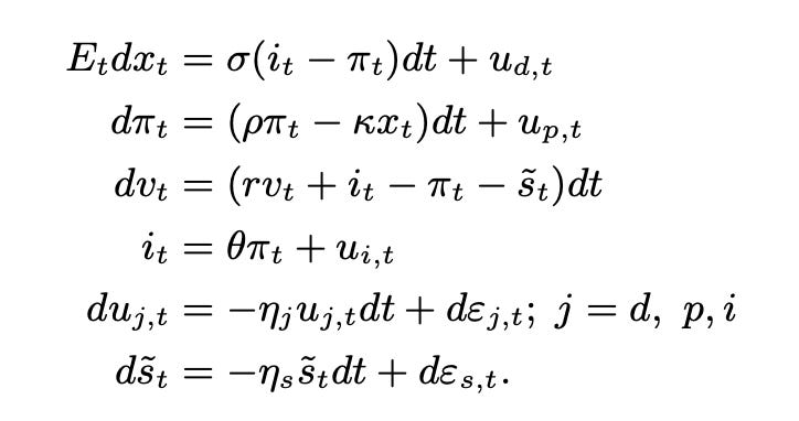
I use theta = 0 and ui = 0 to make these graphs.