Resurrecting the Lucas Phillips Curve

I’ve been remiss about writing here, as I worked full time to finish a new paper. Here it is: Inflation Dynamics with a Generalized Lucas Phillips Curve. It’s a small step in a research program laid out in “Expectations and the Neutrality of Interest Rates.”

There is a chasm between the near uniform beliefs of central bankers, policy analysts, and economists vs. the actual operation of standard economic models in use for 35 years—the new-Keynesian DSGE consensus—on how monetary policy affects inflation. In the standard beliefs, higher interest rates depress aggregate demand, that depresses output and employment, and via the Phillips curve, that depresses inflation, and all of this happens slowly over time, with “long and variable lags.” In the models, higher interest rates raise both inflation and output going forward, allowing only a one-time downward jump at the instant of a shock caused by “equilibrium-selection policy,” and no lag at all.

You will be surprised to learn that there is no simple textbook economic model that describes the uniform beliefs about the basic sign and operation of monetary policy. So I’ve been casting around for alternative models of price stickiness that might bring the models closer to the standard beliefs, with a focus on finding the simplest underlying textbook model that we might build on. You want to get signs right in the simple model before you build on it.

Of course, maybe the models are right and the beliefs are wrong. But it seems worth first exploring whether there is a textbook simple economic model that can embody something like the standard beliefs. That’s the quest.

This paper explores a generalization of the time-honored Lucas (1972) Phillips curve. Lucas wrote that output rises when firms are surprised by higher prices than they expected. That increased output lasts one period, until firms figure out that the higher prices they see are just inflation and not relative demand for their product. But what’s a “period?” I add the idea that different firms sort out aggregate vs. relative demand with different speed. Thus the Phillips curve is

where x is the output gap, p is the price level, and alpha_j is how many firms take length of time j to learn aggregate demand. This is a close relative of Mankiw and Reis’s (2002, 2007) “sticky information” idea, but it turns out to be much simpler to calculate the answers. It’s easy to calculate closed form expressions for the impulse response function using just basic algebra.

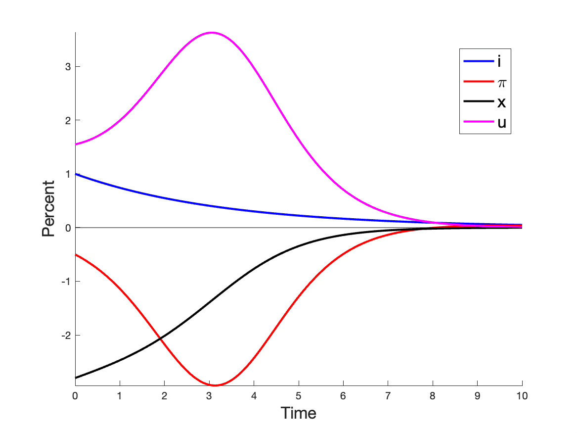
The picture gives a main calculation. The model consists of the above generalized Lucas Phillips curve together with the standard intertemporal IS curve. I feed in the indicated AR(1) interest rate path, along with -0.5% initial disinflation. (Why that’s important is coming up.) Look! Disinflation slowly builds up steam for 3 years, before turning around and fading away.

The Lucas Phillips curve was discarded on the view that it couldn't generate persistent deviations. As you can see, adding heterogeneity gets around that problem. And the Lucas Phillips curve never got in the way of persistent inflation dynamics.

Why is this news? Well, here is the standard model calculation for comparison.

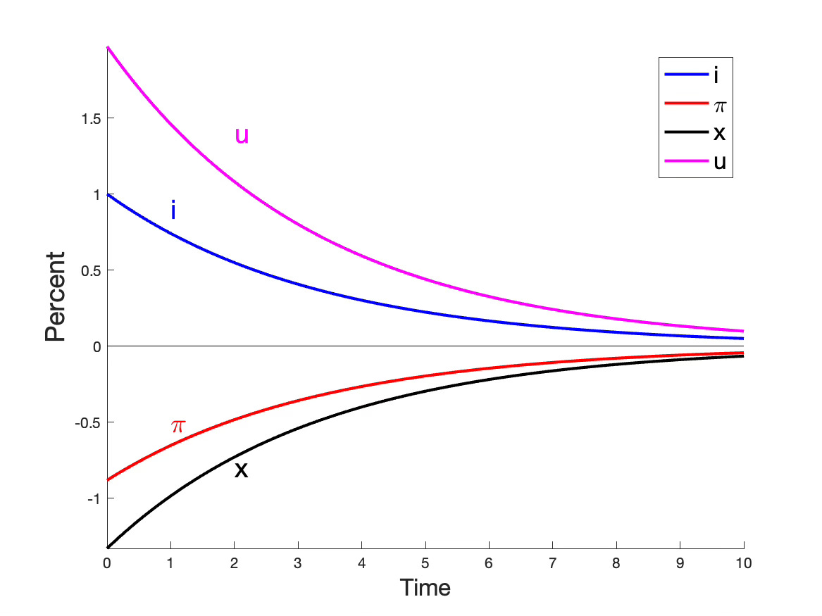
This picture is the standard model with the standard forward looking Phillips curve, together with a Taylor rule interest rate = 1.1 x inflation + disturbance u_t. I reverse-engineer an AR(1) disturbance u_t that produces the same AR(1) interest rate path as the last graph. Inflation and output jump down instantly, but starting 5 minutes after the FOMC meeting at which the higher interest rate is announced, inflation, price level, output growth, and output all rise over time going forward.

Now I think sensible people seeing this kind of result over and over again say, “well, ok, we don’t see downward jumps, but that’s a parable for a process that drags out over time with long and variable lags.” Except you’re not allowed to do that in today’s macroeconomics. The whole point since about 1970 is that we must model the dynamics. Each point in time is an equilibrium. If there is an “adjustment to equilibrium” process, we have to describe it, and describe why smart people don’t profit by adjusting faster.

The plot thickens

The first plot still shows a small downward jump in inflation. I can make it smaller still (see the “double exponential” model in the paper), but not eliminate it totally. And what’s with having to add it as a separate assumption, along with the interest rate path? That turns out to be a second pathology of the standard model which I improve on — we can amplify the initial downward jump — but I don’t totally remove it. The story is revealing about the standard model too, and how utterly different it is from the verbal mechanism (see above) often used, falsely, to describe it.

In response to a shock at time zero, inflation with the generalized Lucas Phillips curve (as plotted in the first graph) is

Sigma, kappa, and an are model parameters; p_0 is the initial price level. Inflation with the standard Calvo-style forward-looking Phillips curve (as plotted in the second graph) is

The lambdas are functions of the same model parameters (sigma, kappa, r), and C is an arbitrary constant.

The form of both equations is the same: inflation is driven by a moving average of interest rates, plus a transient driven by initial conditions. You can use the same equations at time 0 to express the initial condition in terms of initial inflation rather than p_0 and C.

In both cases all the coefficients on the interest rate are positive. Higher interest rates raise inflation.

This shouldn’t be that much of a surprise. (The result is stalking around in a lot of papers if you look for it, though it’s remarkably hidden for a textbook model that’s been around 30 years.) Without pricing frictions, the model reduces to interest rate = constant real rate + expected inflation. So higher interest rate must mean higher expected inflation. To overturn that you’d need the real rate to rise more than one for one with the interest rate, which it doesn’t do. Sticky prices just smooth out the higher inflation prediction over time.

The only hope to get lower inflation with higher interest rates, then, is via the initial term. In the standard model, you need a very negative C, which means a very negative initial inflation, which dies away exponentially. In the modified Lucas model (first equation) you need a small negative p_0, which then can grow more negative over time as the denominator in the first term shrinks. But you still need that negative p_0.

What’s going on, in both models, is that the interest rate path alone (i_t) is not enough to describe the policy environment. There are “multiple equilibria.” That just means that for a given path of interest rates, multiple inflation paths are possible, indexed by p_0 or C in these equations. Thus the policy environment needs to be described not just by the interest rate but also some method of selecting the equilibrium. And, if you want to see lower inflation at the same time as higher interest rates, the equilibrium selection policy does all the work of lowering inflation. Higher interest rates on their own raise inflation.

What is this “equilibrium selection policy?” In the standard new-Keynesian treatment the Fed threatens explosive inflation for all but one initial value. With a rule against explosive solutions, that picks one equilibrium. (The standard Taylor rule plus disturbance folds the selection of initial inflation into the stochastic process for disturbances.) The Fiscal Theory notices that each of these equilibria has different fiscal underpinnings. Notice that the inflation line is below the interest rate line. The real interest rate is a higher real interest cost of the debt. Taxes must rise or spending must fall to pay those higher interest costs. New-Keynesians write a “passive” fiscal policy so that those surpluses always happen. FTPL fixes some element of that fiscal policy, which determines which equilibrium breaks out.

Either way, however, it is the equilibrium-selection/fiscal policy that does all the work of lowering inflation. There is no reason but coincidence that should be associated with higher interest rates. If the Fed has an “equilibrium-selection policy” that will always induce a fiscal contraction, it can just announce lower inflation (pi_0, C), and that lower inflation will happen. It will work even better with lower interest rates.

To be at all a model of monetary policy, we need some reason to tie higher interest rates to lower equilibrium selection/fiscal policy. The last section of the paper does that with the “stepping on a rake” mechanism. With long-term debt and holding fiscal surpluses constant, higher interest rates raise future inflation, but lower current inflation — they give the kick in the pants that makes the whole machinery start.

In that way, we finally have an economically grounded (rational expectations) model that gives something like the standard beliefs of the pattern by which monetary policy affects inflation. It preserves long run neutrality and stability which is a good thing. But neither the standard model nor this modification has anything like the old fashioned mechanism: higher nominal rates are higher real rates that lower output that lowers inflation, even right now and especially not going forward. The standard model is all equilibrium-selection, not aggregate demand. In the fiscal theory interpretation the reduction in aggregate demand comes from fiscal policy. Contra hundreds of papers that use this ancient ISLM intuition to describe equations that work in exactly contrary ways.

Is there an economic model of the standard mechanism? Maybe, but not today. Make a better model.

Is all this nuts? Maybe. Then make a better model.

This is just an investigation of what one ingredient — the Lucas Phillips curve — can do. That’s how we do research. On to the next ingredient.

There are three other approaches that give the same sort of result. First, you can add massive bells and whistles, in the style of the famous models by Christiano, Eichenbaum, and Trabandt. This takes many equations, and deep surgery to the equations of the textbook model. But it cannot be boiled down to something simple, and it too has nothing like the standard mechanism. It too is built on equilibrium-selection not higher interest rates. If dozens of equations and frictions are necessary to produce inflation that goes down going forward, we still admit there is no simple textbook economic model that describes the basic sign of monetary policy.

Second, you can add mechanically backward looking expectations, in effect bringing us back to the 1970s adaptive expectations model. That model describes policy maker intuition quite well, both in the pattern of responses and in the mechanism. But causality may go the other way: policy makers may have played with this model so much they think the world works this way rather than deep historical experience convinces them of the basic story which the model captures. We all tend to view the world through the glasses of received doctrine. More deeply though, it’s not an economic model. If we go this way, we say again that there is no simple textbook economic model that describes the basic sign of monetary policy. Higher interest rates lower inflation only because people are too dumb to catch on and change their expectations of inflation when they see higher interest rates. If they do catch on, game over, the sign flips from negative to positive. Maybe that’s how the world works, but I don’t see anyone at the Fed saying so. I would much prefer that we could start with a basic economic model that describes the sign of monetary policy, and then add bells, whistles, less than perfect expectations, learning, and other frictions to match dynamics if needed. At least it’s worth a search, which is the only way to reassure ourselves that there is no such model.

Third, this model is obviously very close to the Mankiw and Reis “sticky expectations” Phillips curve. It’s a good deal simpler which is its main practical recommendation. Mankiw and Reis admit to complex calculations, and I haven’t found anyone that incorporated their Phillips curve in subsequent model-building. Lesson for the young, you have to make something easy to use. This one is so simple that it’s trivial to incorporate it in other models.

I think this is a nice step, and I hope it’s an ingredient that will inspire others in this general area. If nothing else, it answers my longstanding curiosity about how both Lucas and Mankiw and Reis might work in a model with interest rates rather than money supply targets. I don’t think it’s the final answer, so I’m back to thinking about just how something like adjustment to equilibrium happens slowly over time.

And back to writing for the substack!