
NBER Asset Pricing Lessons

I had the great pleasure of attending the morning session of the NBER Asset Pricing Program at Stanford last Friday. (The afternoon looked just as good, but I couldn’t make it.) A quick review of the three thought-provoking papers I saw. By the way, they were all beautifully presented. Teaching MBAs really does sharpen those public speaking skills!
Kent Daniel presented Inefficiencies in the Security Lending Market joint with Alexander Klos, and Simon Rottke. How about a believable 75% alpha? Yes, 75% per year. Well, -75% per year, but alphas are supposed to be zero. My previous favorite large alpha paper was Owen Lamont’s Go Down Fighting with -2% per month or 24% per year. This was the same idea, but much larger.
The portfolio consists of small, high-priced stocks that cost a lot to short-sell. Hence, though the stock is arguably inefficiently over-priced, there is little that you can do about it, other than not hold such stocks in your portfolio.
You can short-sell most stocks for a small 0.25% per year. But there are often cases in which the cost to short-sell stocks rises dramatically, to hundreds of percent per year. (It’s a daily market, so 1% per day is 365% per year, plus compounding.)
So, Daniel Klos and Rottke form portfolios each month, holding stocks that have the highest short-sale fees. Here’s how the portfolio does:
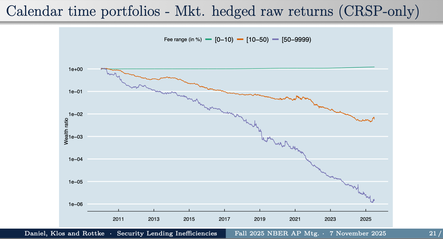
If you hold the portfolio of stocks with 50% per year or more lending fees, a dollar in 2010 is worth 0.0001 cents in mid 2025. Efficient markets say you shouldn’t be able to make money on the stock market. But you shouldn’t be able to systematically lose money either, except by paying too many fees.
Here is the kicker: The same portfolio, but adding back in the fees. Suppose you held those stocks, but lent them out and got the full fee:
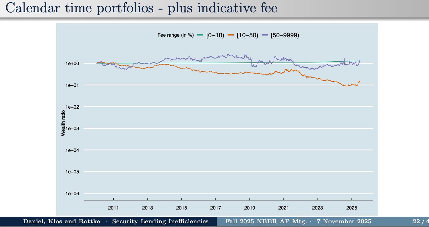
Zero. The fee exactly balances the loss of value of the stock.
Daniel Klos and Rottke also document that close to half of the fee gets swallowed up in the intermediary chain of lending agents and prime brokers that handle the transactions, and they add a lot of great detail on the shorting market.
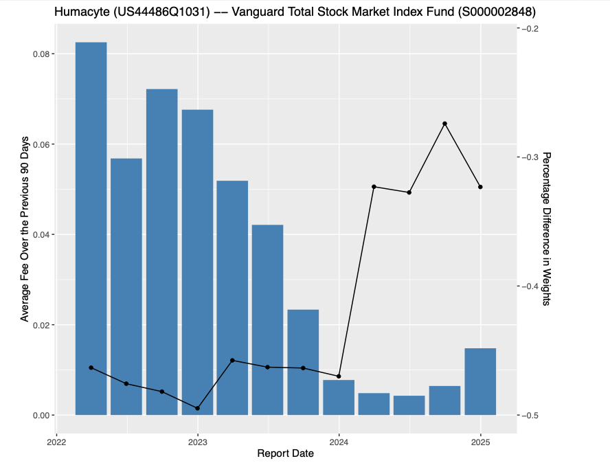
What can you do? At a minimum, don’t hold such stocks. Who holds such ridiculously overpriced stocks? Well, to some extent, all of us. If you have an index fund that is pledged to hold the index, you hold them too. Daniel Klos and Rottke show that index funds with some latitude lower their weights as well as lend out shares, but not all can do so.
There was an interesting discussion whether extreme short-selling fees have gotten worse over time. They have in the data reported by Daniel et al.
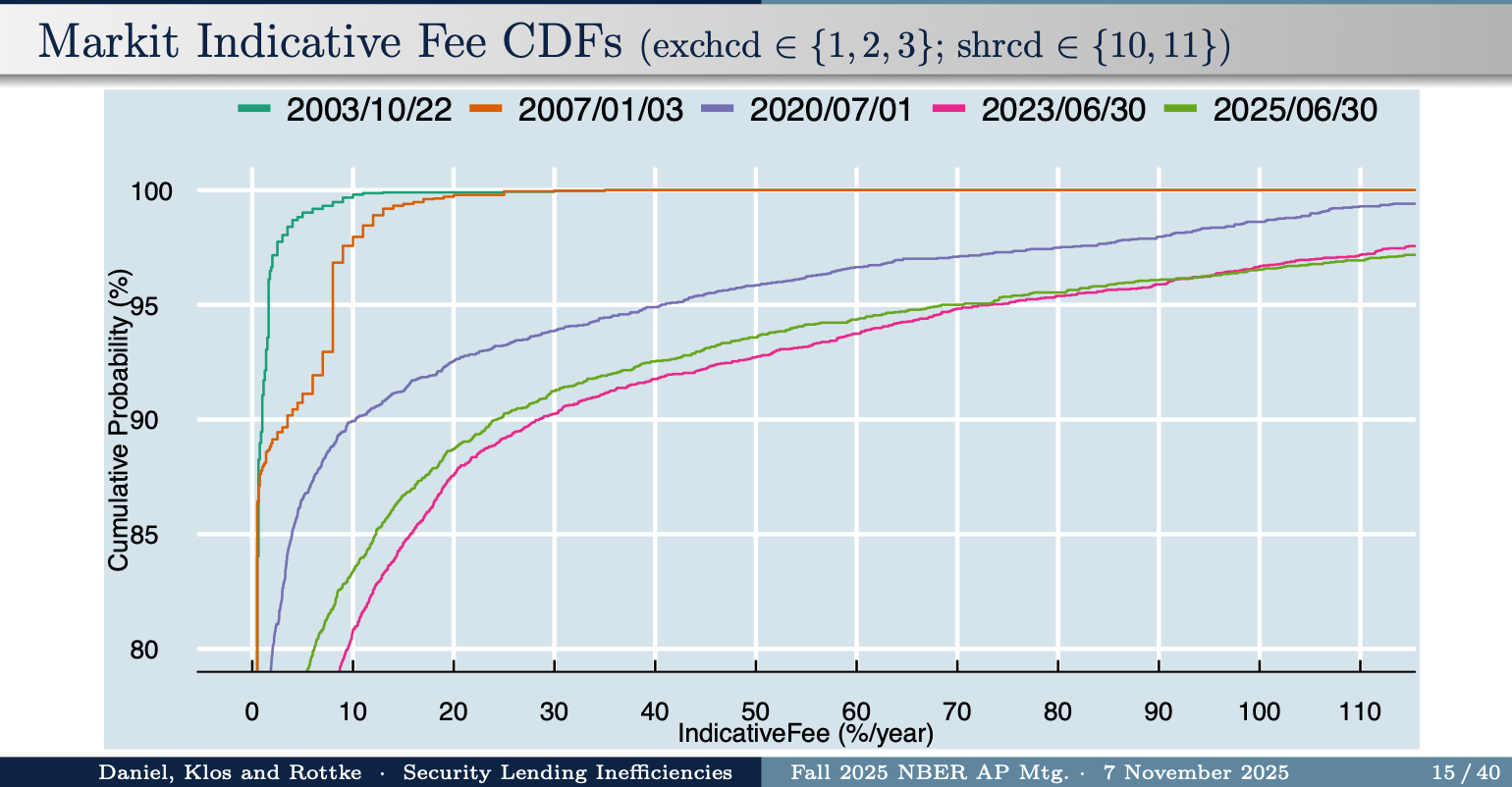
This is the cumulative distribution of fees, so the steady downward drift is a steady rightward drift in fees. Discussant Matthew Ringgenberg (a great discussion with lots of detail on the shorting market) pointed out that could be because it’s now possible to short sell many stocks that previously couldn’t be shorted at all. When a new cancer drug is approved, which costs $100,000 per year, the cost of treating that cancer goes down from infinity to $100,000, not up. But that interesting discussion does not detract at all from Daniel et al’s real time strategy.
****
Aditya Chaudhry presented Endogenous Elasticities: Price Multipliers Are Smaller for Larger Demand Shocks coauthored with Jiacui Li , with a great discussion by Valentin Haddad.
“Downward sloping demand curves” are a big rage in finance. Li and Chaudhry divided popular measures of “demand” shocks by size. Most shocks are small, less than 1% of shares outstanding. They have surprisingly large marginal effects; the price changes by about twice the change in quantity. They subdivide shocks by size, and find that the elasticity for large shocks is smaller. One example:
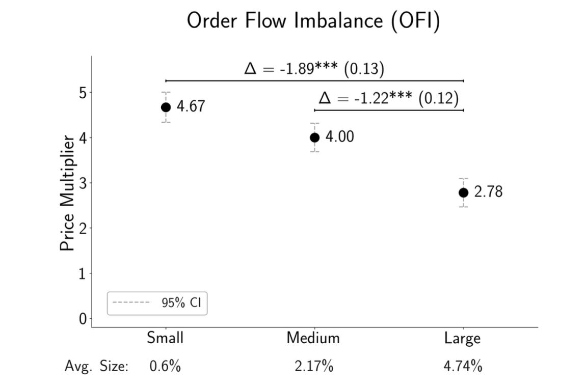
This finding tells us a lot about what the mechanism is. A natural conclusion: It isn’t worth people’s time on the other side of the trade to arbitrage 1% price rises, but maybe it is once prices rise more than that.
This kind of matching theories with basic facts, rather than attempt encompassing “tests” is often worthwhile.
A common fact helps to understand both papers: Large persistent price inefficiencies are small expected return inefficiencies. P/D=1/(r-g) so r = g+D/P. The elasticity of D/P with respect to P is also D/P (Pd(D/P)/dP=-D/P), so at a dividend yield of 1.5% (S&P500 is now less than that), a 1% permanent rise in price lowers the return by 1.5% of 1%, i.e. 1.5 basis points. Sitting that one out might be excusable. Even the aforementioned 25 bp cost of short selling means it is not worth arbitraging a price until it is 17% too high.
****
Next, Haven’t We Seen This Before? Return Predictions from 200 Years of News by AJ Yuan Chen, Gerard Hoberg, and Miao Ben Zhang, with a superb discussion by Svetlana Bryzgalova. “History doesn’t repeat itself, but it often rhymes” is the introductory quote.
Here is my interpretation: Big data in economic forecasting faces a N»T problem. We have far more signals than we have non-overlapping time periods to evaluate how those signals work. You can’t just run regressions R(t+1) = beta’ x(t) + error and forecast with E[R(t+1)|x(t)] - beta’x(t) when there are more x’s (N) than there are ts (T).
But we can look for time periods in which the x’s are “close to” today's x, and see the average outcomes after those, and we can do that no matter how large the x. If your question is forecasting, not estimation (of beta), then the experience of “nearby” x(t) can tell you E[R(t+1)|x(t)] directly. Chen Hoberg and Zhang do that. They look at newspaper text data to find the 5 months “most like” the current one, and then forecast stock returns and macroeconomic variables by their average value in the subsequent one.
Bryzgalova gave a master class in econometrics pointing out some of the issues. A few things I learned: (I don’t do big data. This is probably all simple for those of you who do.) This is after all nonparametric estimation, with a well known bias vs. variance issue, and slow convergence. For large dimensional x it is a bad idea to define “distance” by euclidean norm. As the number of dimensions grows, basically everything is very far from everything else. The paper uses the cosine of the angle between x and y as the definition of distance. Bryzgalova suggested the arccos (cosine(x,y)), i.e. the angle itself, as a better measure, which obeys the triangle inequality. Both measures lose the scale of x however. Also, the “most similar” last 5 episodes are the same for every forecasting variable. Thus, the technique does not let the data find that, say, price-earnings ratios are useful for forecasting stock returns, while batting averages are useful for forecasting World Series winners. There was a discussion that therefore the dictionary of terms matters a lot to the results. They excluded sports articles for a reason.
I was similarly taken with Kelly Malamud and Zhou’s finding that one should just go ahead and run regressions with N»T, but regularize by holding down the size of the coefficients. That technique also imposes that all the right hand variables are roughly of the same importance, and thus the choice of variables and units matters.
I’m not sure anyone was ready to go out and trade on the forecasts. As a colleague sitting next to me whispered during an earlier paper, if there was even one tenth the alphas in financial markets than one finds in every one of these conferences, we’d all be rich. But the question how to deal with huge data is with us, and I learned a lot.
Apologies to the other authors. The papers all looked fascinating, but I had an errand that couldn’t be put off.
Jim Scott and I studied this 15 years ago using prices we obtained (and archived in real time) from our prime brokers and found precisely the same result - for the same reasons. One small point is that these tend to be very thinly traded stocks so illiquidity also plays a role here.
Explain how Nancy Pelosi was able to consistently beat the Dow by a huge margin, if you can.