
Fiscal Tidbits, Part 1

A few fiscal theory related tidbits came up in the last few weeks. I’m still in the mode of story telling in advance of formal models, but vaguely plausible stories are a vital first step.
Surplus/GDP or Surplus/Debt?
The 1960s saw inflation emerge. Even the conventional story links that to fiscal policy, Johnson’s desire to spend for the Vietnam War and Great Society at the same time. (Trade deficits and the failure of Bretton Woods are, I think, an overlooked part of the story as well.) The trouble is that deficits were small relative to GDP, at least relative to what we routinely see today with less inflation.
As a reminder, here is inflation from the 1960s to the 1980s
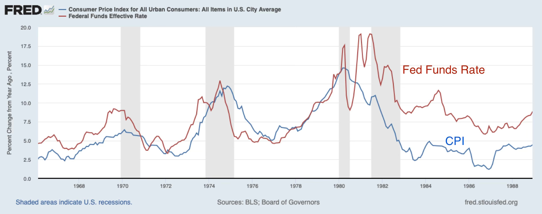
Here are primary surpluses relative to GDP
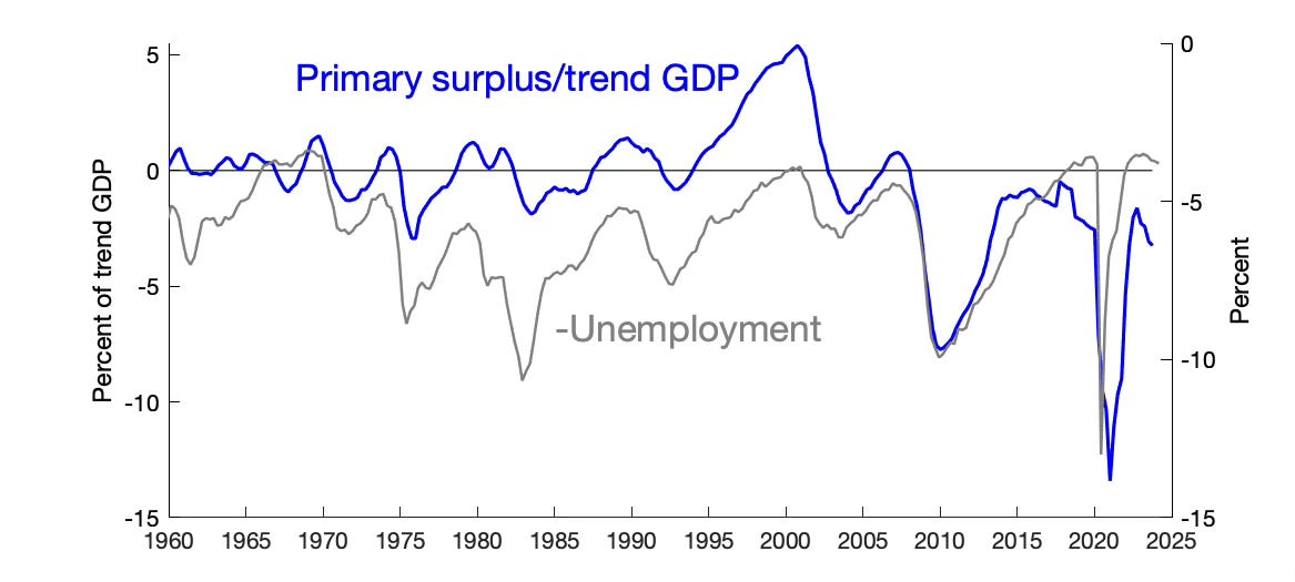
(Surplus is net lending or borrowing, AD02RC1Q027SBEA, primary surplus subtracts interest payments A091RC1Q027SBEA.) You can see there are deficits in the late 1960s and early 1970s, and they are suggestively linked to the surges of inflation. 1975 was unprecedented in peacetime. But even 3% of GDP is small compared to the 2008 deficit, which produced no inflation.
Chris Sims “Origins of US Inflation since 1950” points out, correctly, that what matters for inflation is unfunded deficits relative to debt, not relative to GDP. Other things constant, more debt means that the same deficit has less inflationary impact.
In equations,
B is nominal debt, P is the price level, s is the real primary surplus and beta is the discount factor. The percentage change in the price level P depends on the percentage change in s/B, the surplus to debt ratio. Starting at t+1, and rearranging,
unexpected inflation is driven by the revision in unfunded deficits relative to the real value of debt.
Yes, more debt means that deficits have less inflationary effect. At 100% debt to GDP, 1% inflation inflates away 1% of GDP debt and pays for a 1% of GDP unfunded deficit. At 200% debt to GDP, 0.5% inflation inflates away the same 1% of GDP unfunded deficit. A $1000 loss lowers Tesla’s stock price by 1/557,160,000. It lowers the value of a $2,000 food truck business by 50%. More debt is a buffer against fiscal shocks.
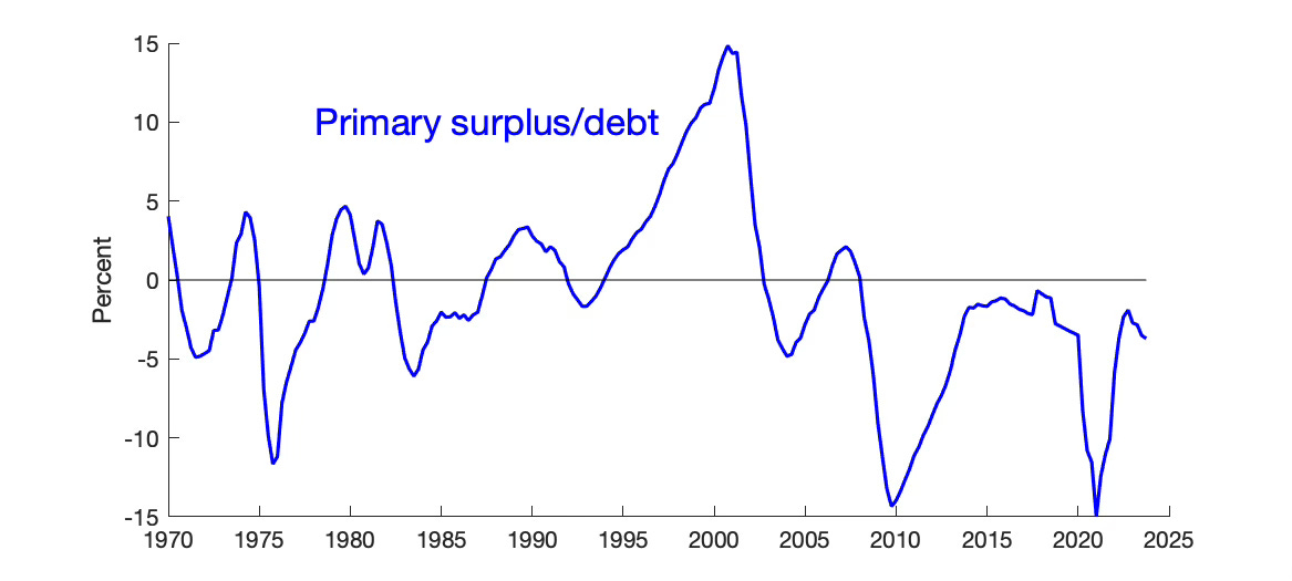
When we look at the history of US surplus relative to debt, the picture changes. 1972 is as inflationary as 2008, and 1975 was almost as bad as 2022. Now we are starting to see deficits of comparable size to the inflation that followed! (I use Federal Debt held by the Public, FYGFDPUN. Sadly Fred only has it starting in 1970.)
Of course 2008 did not produce inflation. Fiscal theory does not say that deficits cause inflation. It only says that the fraction of deficit people do not expect to be paid back, either by higher future surplus or by lower future interest costs, is inflationary. 2008 got, I think, really lucky with low interest costs, and to its credit (or maybe not, if you wanted stimulus), the Obama Administration always promised eventual debt reduction.
The main point, however, is that unfunded surpluses relative to debt measure their inflationary impact, and other things constant, more debt is better. Likewise more domestic and less foreign debt means inflation is more insulated against surplus shocks.
But your intuition still says that countries or times with a lot of debt should be in more trouble. The small deficits of the early 1970s relative to GDP should not have inflated such a large country, no?
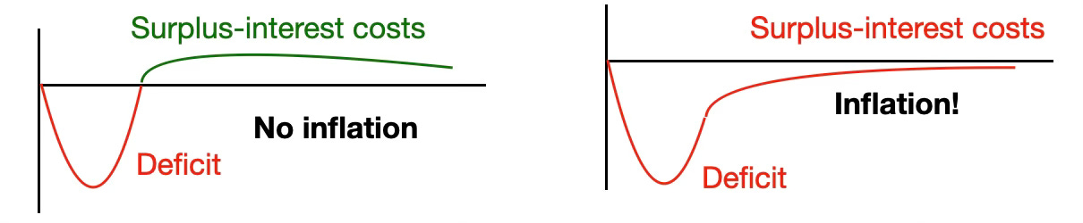
I think the reason for your intuition is that a country with small debt, and thus small requirements for future surpluses, should have an easier time raising surpluses to pay off deficits, and thus avoid inflation. It should have an easier time promising the left possibility above, rather than the right one.
But if it does not do so, then small unfunded deficits relative to a small debt cause more inflation. More initial debt gives less inflation given the surplus shock. Your intuition just says that the present value surplus shock should be smaller if there is less initial debt.
This is the main point of this section of the post. To reiterate, surpluses relative to debt drive inflation. Given deficits and expected surpluses, more debt means less inflation. Your intuition about debt being bad is also correct, because it typically means it will be harder for a country to promise future surpluses to pay off deficits. Beware in reading history, or judging whether more debt makes inflation more likely, just what is actually held constant and what is not.
Now, the question of the 1970s becomes the opposite of 2008. Why did people not trust that such “small” deficits would be repaid? That leads us to productivity slowdown, political polarization, and malaise. Sims has a good story for 1975 vs. 1980, that the high interest costs of 1980 provoked the fiscal tightening that you see unfold dramatically. The present value of surpluses really did rise in 1980! But we’ll leave that story telling for later. The point for now, is just that the small deficits of the early 1970s, if unfunded, could have produced such a large inflation, because paradoxically debt was smaller.
This lesson matters today. I’m going to the Bank of Japan later this month, so the question why did Japan have less covid inflation than us comes up. One answer is — they have (a lot) more debt, so the percent increase in debt of a given unfunded deficit is smaller. They also had smaller deficits. More later.
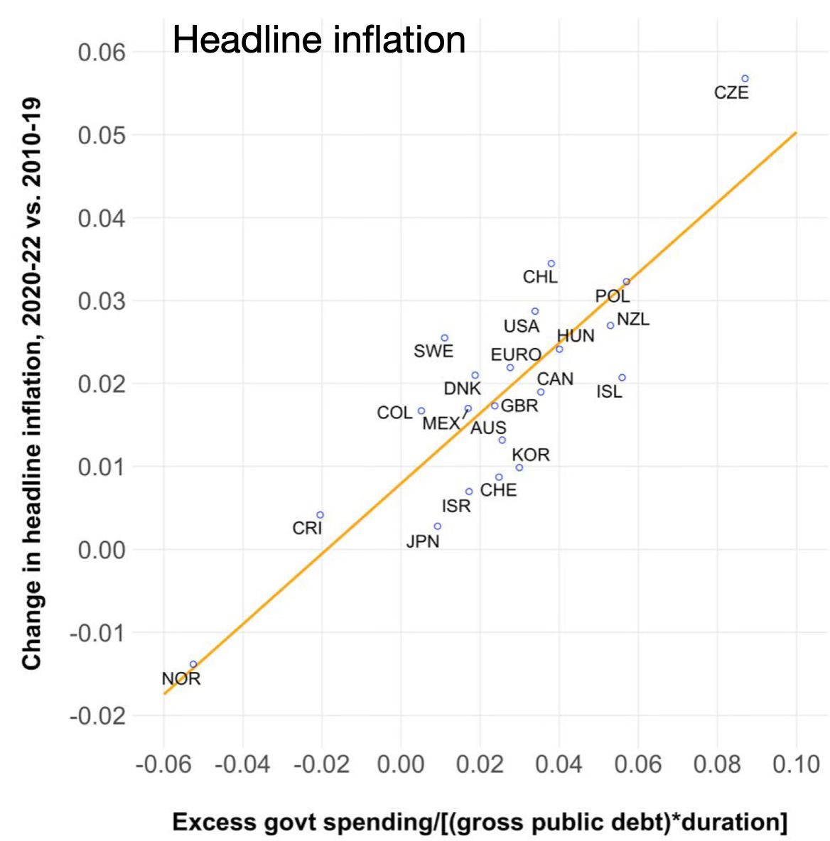
This graph comes from Barro and Bianchi. Covid spending lines up nicely with inflation, if you scale by debt. Spending relative to debt drives inflation. Japan (which actually had a bit more inflation than the graph says because it came later) has a lot more debt to dilute its deficits! The line represents an ideal in which each country is expected to repay the same fraction of that spending, about half.
Update: This point implies an important weakness in the usual linearization. When linearizing, I divide the surplus by the steady state or average debt. Clearly, surpluses matter more when debt is smaller. There is an interaction term, which my linearization misses.
Primary or total deficits?
Fiscal theory has been confusing, because it points to primary not total deficits. Just why do interest costs on the debt not matter? They do, and I only now have a different perspective on the same old equations I’ve been playing with for 30 years.
I usually start with the one period debt case,
The price level adjusts so the real value of debt equals the present value of primary surpluses, discounted by the return on the government debt portfolio. (You can’t always substitute that return for the proper marginal utility discounter, but I assume here that the expected return is large enough that you can.) This leads one to see a separation between primary surplus, the “cash flow,” and interest costs on the debt, properly measured, which act as a “discount rate.” The “discount rate” term matters a lot empirically.
The linearized version of the same formula lets us subtract rather than divide by interest costs,
v is the log real value of debt, s tilde is the ratio of surplus to debt, and r is the real return. Here you see that interest costs on the debt act just like a primary deficit. For my intuition, I am starting to think less as an asset pricer, in terms of present values and discount rates, and more in flow terms, interest costs on the debt and primary surpluses and deficits.
The interest cost is important. 1% interest rate means 1% of GDP primary deficit at 100% debt to GDP. It means 2.5% primary deficit at 250% debt to GDP. That’s a reason that, contrary to last point, more debt means more inflation danger. It means more exposure to interest rate changes.
What just occurs to me, though is that s-r is the total deficit, including interest costs. So we can express fiscal theory, to the approximation that subtracting is the same as dividing, to say that the price level adjusts so that the real value of debt equals the total deficit, discounted at a constant (rho, here) rate.
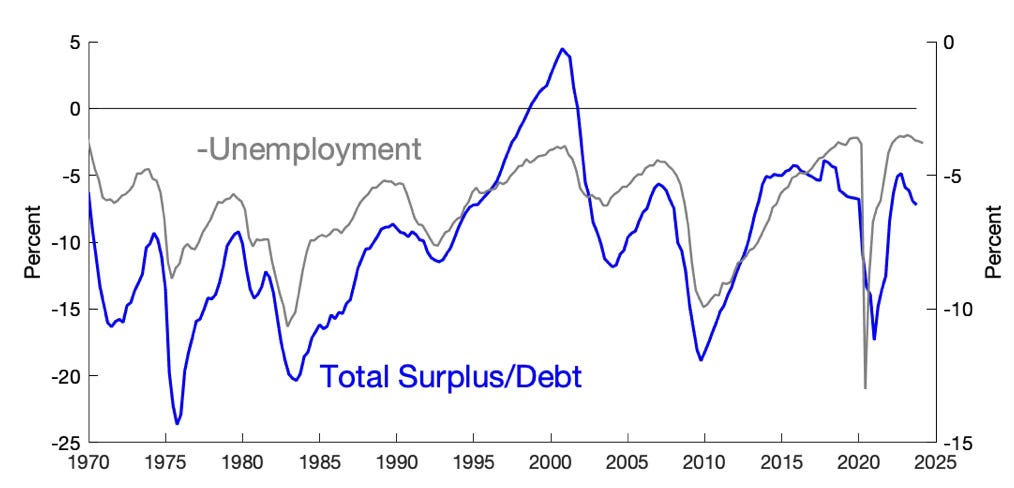
The plot of total deficit looks even worse. Ignore here the fact that the average is negative. The linearized formula describes deviations from steady state, not the level. But on this basis, the 1970s really are comparable to 2022.
(I include unemployment in these graphs, made for other purposes, to remind people that surpluses and deficits are overwhelmingly driven by the state of the economy, not changes in tax or spending legislation. Those however move the permanent component of surplus, much smaller and harder to see, but crucial for expected repayment.)
Not sure if I'm missing something, but I think your "primary surplus/gdp" graph is wrong. You say "Surplus is net lending or borrowing, AD02RC1Q027SBEA, primary surplus subtracts interest payments A091RC1Q027SBEA" But if I take the first series minus the second, I don't get that. I get this: https://fred.stlouisfed.org/graph/?g=1o5sF It is never positive.
Finally, I ADDED the two series and divided by real GDP (GDPC1) although most measures or real or potential real look the same... and I get a graph that looks like yours. Here's the link: https://fred.stlouisfed.org/series/AD02RC1Q027SBEA#0 .
If your graph has them added, then the comments/stories around it are off too.
I suspect my graph with them subtracted isn't right because we did indeed run primary surpluses in the late 1990s... but what data to look at?
Any thoughts?
I'm very interested in finding good data to play with and think about FTPL. So, I'd be interested in any suggestions on good time series for real primary surpluses or appropriate measures of debt, etc. I plan to look at these globally over the summer, but wanted to start with the best data I know of which is USA FRED data so I feel confident that I'm looking at what I want to look at then I can worry about non-US measures.
Thanks.
Barro's graph is quite impressive. However, he does not include monetary phenomenon.
Most if not all of those countries had both expansive fiscal and monetary policies.
Shouldn't both be included?